6. 曲面问题 Surface Problems#
本章内容
本章处理嵌入高维空间的流形网格上的偏微分方程. 以平面闭曲线的平均曲率流为例, 介绍 Barrett–Garcke–Nürnberg (BGN) 参数化有限元格式的 Firedrake 实现, 并在收缩圆、二维哑铃形曲线和三维哑铃面三个算例上检验半径与面积的演化以及颈部掐断现象.
Overview
This chapter treats partial differential equations on manifold meshes embedded in a higher-dimensional space. Using mean curvature flow of a closed planar curve as the example, it presents a Firedrake implementation of the parametric finite element scheme of Barrett–Garcke–Nürnberg (BGN) and verifies the radius and area evolution as well as the neck-pinch phenomenon on a shrinking circle, a planar dumbbell curve, and a three-dimensional dumbbell surface.
6.1. 平均曲率流 Mean curvature flow#
平均曲率流使曲面沿其平均曲率向量演化. 对平面中的闭合曲线 \(\Gamma(t)\), 取外法向 \(\nu\), 并令曲率的符号约定为 \(\kappa=-1/R\) (半径为 \(R\) 的圆), 则
Mean curvature flow evolves a surface along its mean-curvature vector. For a closed planar curve \(\Gamma(t)\), let \(\nu\) be the outer normal and use the convention \(\kappa=-1/R\) for a circle of radius \(R\). Then
其中 \(V\) 是外法向速度. 因而圆满足 \(R(t)^2=R(0)^2-2t\), 会在有限时间收缩到一点. 下面实现 Barrett–Garcke–Nürnberg (BGN) 的参数有限元格式 [BGNurnberg07]. 它同时求下一时刻的曲线参数化 \(X^{m+1}\) 和标量曲率 \(\kappa^{m+1}\); 切向自由度由第二个方程决定, 通常能维持良好的顶点分布.
Here \(V\) is the outer normal velocity. Hence a circle satisfies \(R(t)^2=R(0)^2-2t\) and collapses to a point in finite time. The following implements the parametric finite element scheme of Barrett–Garcke–Nürnberg (BGN) [BGNurnberg07]. It solves simultaneously for the next curve parametrization \(X^{m+1}\) and scalar curvature \(\kappa^{m+1}\); the second equation determines the tangential degrees of freedom and usually maintains a good vertex distribution.
对任意标量检验函数 \(\chi\) 和向量检验函数 \(\eta\), 格式为: For every scalar test function \(\chi\) and vector test function \(\eta\), the scheme is:
上标 \(h\) 表示顶点质量集总内积, 可按第 1 章数值积分一节的方法构造自定义求积规则实现: 下面的 vertex_quadrature 为区间和三角形单元统一构造顶点求积, 因而同一份实现既适用于平面曲线, 也适用于 \(\mathbb R^3\) 中的曲面. CellNormal 需要先由一个连续、非零的参考法向场定向. 函数 evolve_mcf 封装该格式: 变分问题和求解器在时间循环外构造, 循环内求解并更新网格坐标, 同时记录界面测度 (曲线周长或曲面面积)、由散度定理给出的包围测度 (面积或体积) \(\frac1d\oint_{\Gamma_h}X\cdot\nu\,\mathrm{d}s\) (\(d\) 为空间维数) 以及指定时刻坐标场的深拷贝. 这些量都是并行安全的: assemble 是集合操作, 快照以 Function 返回, 并行时可直接交给 VTKFile 输出; 本章用 matplotlib 从快照中取顶点坐标绘图, 与全书一样假定笔记本串行执行. 本章的算例都调用 evolve_mcf.
The superscript \(h\) denotes the vertex mass-lumped inner product, implemented here through a custom quadrature rule as in the numerical-integration section of Chapter 1: vertex_quadrature below constructs the vertex rule for interval and triangle cells alike, so the same implementation works for planar curves and for surfaces in \(\mathbb R^3\). CellNormal must first be oriented by a continuous nonzero reference normal field. The function evolve_mcf encapsulates the scheme: the variational problem and solver are constructed outside the time loop, and inside the loop we solve, update the mesh coordinates, and record the interface measure (curve length or surface area), the enclosed measure (area or volume) \(\frac1d\oint_{\Gamma_h}X\cdot\nu\,\mathrm{d}s\) (with \(d\) the spatial dimension) given by the divergence theorem, and deep copies of the coordinate field at selected times. All of these are parallel safe: assemble is collective, and the snapshots are returned as Function objects that can be written directly with VTKFile in parallel. The matplotlib plots in this chapter extract vertex coordinates from the snapshots and, as everywhere in this book, assume serial notebook execution. All examples in this chapter call evolve_mcf.
from firedrake import *
import matplotlib.pyplot as plt
import numpy as np
import FIAT
import finat
from mpi4py import MPI

def vertex_quadrature(mesh):
    """Vertex quadrature rule (mass lumping) for interval/triangle cells."""
    cell_name = mesh.ufl_cell().cellname
    if cell_name == 'interval':
        ref_cell = FIAT.reference_element.UFCInterval()
        weights = [1/2, 1/2]
    elif cell_name == 'triangle':
        ref_cell = FIAT.reference_element.UFCTriangle()
        weights = [1/6, 1/6, 1/6]
    else:
        raise ValueError(f'unsupported cell: {cell_name}')
    point_set = finat.quadrature.PointSet(ref_cell.vertices)
    qrule = finat.quadrature.QuadratureRule(point_set, weights)
    qrule.ufl_signature = repr(qrule)
    return qrule

def evolve_mcf(mesh, time_step, num_steps, snapshot_steps=()):
    """Evolve the mesh by the BGN scheme and record diagnostics."""
    dim = mesh.geometric_dimension
    V = FunctionSpace(mesh, 'CG', 1)
    V_vector = VectorFunctionSpace(mesh, 'CG', 1, dim=dim)
    W = V_vector * V

    X, kappa = TrialFunctions(W)
    eta, chi = TestFunctions(W)
    normal = CellNormal(mesh)
    vertex_dx = dx(scheme=vertex_quadrature(mesh))

    a = (
        inner(X, chi*normal)*vertex_dx
        - time_step*kappa*chi*vertex_dx
        + kappa*inner(normal, eta)*vertex_dx
        + inner(grad(X), grad(eta))*dx
    )
    L = inner(mesh.coordinates, chi*normal)*vertex_dx

    solution = Function(W)
    X_next, kappa_next = solution.subfunctions
    problem = LinearVariationalProblem(a, L, solution)
    solver = LinearVariationalSolver(
        problem, solver_parameters={'ksp_type': 'preonly', 'pc_type': 'lu'}
    )

    x = SpatialCoordinate(mesh)
    enclosed_form = 1/dim*inner(x, normal)*dx
    times = [0.0]
    measures = [assemble(1*dx(domain=mesh))]
    enclosed = [assemble(enclosed_form)]
    snapshots = {0.0: mesh.coordinates.copy(deepcopy=True)}
    for step in range(1, num_steps+1):
        solver.solve()
        mesh.coordinates.assign(X_next)
        times.append(step*time_step)
        measures.append(assemble(1*dx(domain=mesh)))
        enclosed.append(assemble(enclosed_form))
        if step in snapshot_steps:
            snapshots[step*time_step] = mesh.coordinates.copy(deepcopy=True)

    return {'times': np.asarray(times), 'measures': np.asarray(measures),
            'enclosed': np.asarray(enclosed), 'snapshots': snapshots}
提示: 内置的集总求积 Tip: built-in lumped quadrature
顶点求积也可用内置的 KMV 积分公式得到, 即 dx(scheme='KMV', degree=1) 在区间和三角形单元上都与上面的自定义公式一致. 这里 'KMV' 也可写为其别名 'lump', 且这两个名字不区分大小写 ('default' 和 'canonical' 则区分). 注意必须显式指定 degree=1: 若省略, 会按形式的估计次数选取更高阶的集总规则, 结点更多, 不再是顶点求积. scheme 参数的官方说明见 Quadrature rules.
The vertex quadrature can also be obtained from the built-in KMV quadrature rules: dx(scheme='KMV', degree=1) agrees with the custom rule above on both interval and triangle cells. Here 'KMV' may also be written as its alias 'lump', and these two names are case-insensitive (whereas 'default' and 'canonical' are case-sensitive). Note that degree=1 must be given explicitly: if omitted, a higher-order lumped rule is chosen according to the estimated degree of the form, with more nodes, and is no longer the vertex rule. The scheme argument is documented on the Quadrature rules page.
6.1.1. 收缩圆 A shrinking circle#
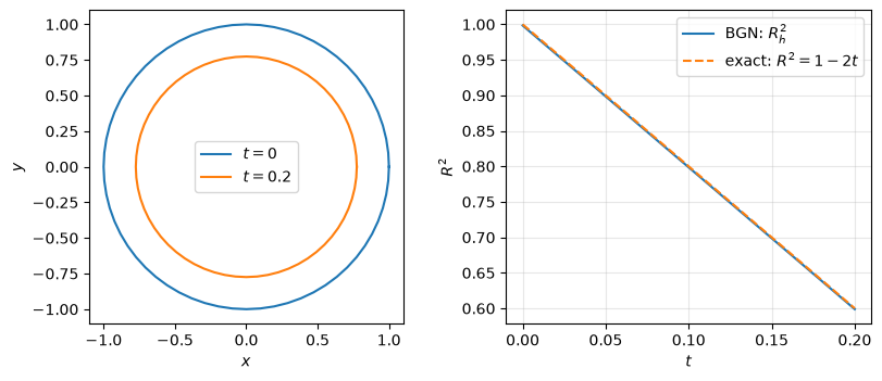
初始曲线取单位圆, 精确解满足 \(R(t)^2=1-2t\). 对初始圆, 坐标场就是外向的参考法向场, 可直接用于定向 CellNormal. 离散半径平方由包围面积计算: \(R_h^2=A_h/\pi\). 内接多边形的面积略小于圆的面积, 因而 \(R_h^2(0)\approx0.9984\) 而非 \(1\).
The initial curve is the unit circle, for which the exact solution satisfies \(R(t)^2=1-2t\). For the initial circle, the coordinate field itself is an outward reference normal field and can be used directly to orient CellNormal. The discrete squared radius is computed from the enclosed area, \(R_h^2=A_h/\pi\). The area of the inscribed polygon is slightly smaller than that of the circle, so \(R_h^2(0)\approx0.9984\) rather than \(1\).
mesh_circle = CircleManifoldMesh(64, radius=1.0)
mesh_circle.init_cell_orientations(SpatialCoordinate(mesh_circle))

circle_step = 1.0e-3
circle_steps = 200
result_circle = evolve_mcf(mesh_circle, circle_step, circle_steps,
                           snapshot_steps=(circle_steps,))
radius_squared = result_circle['enclosed']/np.pi
exact_final = 1 - 2*circle_steps*circle_step
print(f'final R_h^2 = {radius_squared[-1]:.4f}, exact = {exact_final:.4f}')
assert abs(radius_squared[-1]-exact_final) < 5e-3
final R_h^2 = 0.5988, exact = 0.6000
左图为初始与终止时刻的曲线, 收缩过程中保持接近圆形; 右图中 \(R_h^2\) 沿精确直线下降, 实测中与 \(1-2t\) 的最大偏差约为 \(1.6\times10^{-3}\).
The left plot shows the initial and final curves, which remain close to circular while shrinking; on the right, \(R_h^2\) decreases along the exact line, with a maximum deviation from \(1-2t\) of about \(1.6\times10^{-3}\) in our tests.
fig, axes = plt.subplots(1, 2, figsize=(8, 3.4), constrained_layout=True)
for t in sorted(result_circle['snapshots']):
    points = result_circle['snapshots'][t].dat.data_ro
    closed_points = np.vstack((points, points[0]))
    axes[0].plot(closed_points[:, 0], closed_points[:, 1], label=f'$t={t:g}$')
axes[0].set_aspect('equal')
axes[0].set_xlabel('$x$')
axes[0].set_ylabel('$y$')
axes[0].legend()

axes[1].plot(result_circle['times'], radius_squared, label='BGN: $R_h^2$')
axes[1].plot(result_circle['times'], 1-2*result_circle['times'], '--',
             label='exact: $R^2 = 1 - 2t$')
axes[1].set_xlabel('$t$')
axes[1].set_ylabel('$R^2$')
axes[1].grid(alpha=0.3)
_ = axes[1].legend()
6.1.2. 哑铃形曲线 A dumbbell-shaped curve#
第二个算例取极坐标下的哑铃 (花生) 形初始曲线
两端粗、中间细. 代码将圆网格的顶点按该参数化重新布点, 再用位置场定向 CellNormal: 星形曲线上位置向量与外法向的内积为正, 因而位置场仍是合法的参考法向场.
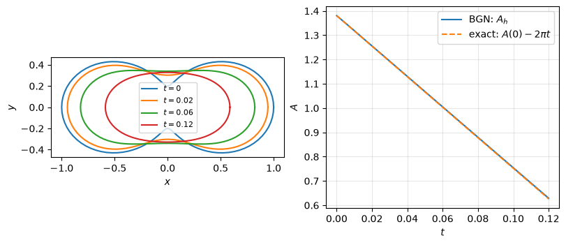
由 Gage–Hamilton 与 Grayson 的定理 [GH86, Gra87], 嵌入的平面闭曲线在平均曲率流下先变凸, 随后渐近于圆并在有限时间收缩为一点; 与三维哑铃曲面不同, 平面曲线不会发生颈部掐断; 三维情形的掐颈见下一小节. 光滑流的包围面积精确满足 \(A(t)=A(0)-2\pi t\), 下面以它作为定量检验; 周长则单调下降.
The second example starts from the dumbbell (peanut) shaped curve given in polar coordinates by
with two thick lobes and a thin waist. The code repositions the vertices of the circle mesh according to this parametrization and then orients CellNormal with the position field: on a star-shaped curve the inner product of the position vector with the outer normal is positive, so the position field is still a valid reference normal field.
By the theorems of Gage–Hamilton and Grayson [GH86, Gra87], an embedded closed planar curve under mean curvature flow first becomes convex, then approaches a circle and shrinks to a point in finite time; unlike the three-dimensional dumbbell surface, a planar curve develops no neck pinch; the pinching case is shown in the next subsection. For the smooth flow the enclosed area satisfies \(A(t)=A(0)-2\pi t\) exactly, which we use below as a quantitative check; the length decreases monotonically.
num_vertices = 128
mesh_dumbbell = CircleManifoldMesh(num_vertices, radius=1.0)
coords = mesh_dumbbell.coordinates.dat.data_ro
theta = np.arctan2(coords[:, 1], coords[:, 0])
radius_dumbbell = 0.6 + 0.4*np.cos(2*theta)
mesh_dumbbell.coordinates.dat.data[:, 0] = radius_dumbbell*np.cos(theta)
mesh_dumbbell.coordinates.dat.data[:, 1] = radius_dumbbell*np.sin(theta)
mesh_dumbbell.init_cell_orientations(SpatialCoordinate(mesh_dumbbell))

dumbbell_step = 5.0e-4
dumbbell_steps = 240
result_dumbbell = evolve_mcf(
    mesh_dumbbell, dumbbell_step, dumbbell_steps,
    snapshot_steps=(40, 120, dumbbell_steps),
)
areas = result_dumbbell['enclosed']
areas_exact = areas[0] - 2*np.pi*result_dumbbell['times']
max_area_deviation = np.max(np.abs(areas-areas_exact))
print(f'initial area = {areas[0]:.4f} '
      f'(continuum 0.44*pi = {0.44*np.pi:.4f})')
print(f'length: initial = {result_dumbbell["measures"][0]:.4f}, '
      f'final = {result_dumbbell["measures"][-1]:.4f}')
print(f'max |A_h - (A_h(0) - 2*pi*t)| = {max_area_deviation:.2e}')
assert max_area_deviation < 5e-3
assert np.all(np.diff(result_dumbbell['measures']) < 0)
initial area = 1.3805 (continuum 0.44*pi = 1.3823)
length: initial = 5.1948, final = 2.9832
max |A_h - (A_h(0) - 2*pi*t)| = 2.27e-03
左图的快照显示, 颈部的凹陷首先被抹平, 曲线先变凸, 再逐渐趋圆并收缩; 右图中离散面积与精确直线几乎重合, 实测中最大偏差约为 \(2.3\times10^{-3}\), 周长从 \(5.19\) 单调降到 \(2.98\).
本章的算例都直接修改 mesh.coordinates, 因而每一步的积分和 CellNormal 都在更新后的多边形曲线上计算. 若后续需要把移动网格交给 DMPlex 自适应操作, 还须将坐标同步到底层 DMPlex, 见 更新 DMPlex 中的网格坐标 Updating mesh coordinates in DMPlex.
The snapshots in the left plot show that the concave neck is smoothed out first, the curve becomes convex, and it then approaches a circle while shrinking; on the right, the discrete area nearly coincides with the exact line, with a maximum deviation of about \(2.3\times10^{-3}\) in our tests, while the length decreases monotonically from \(5.19\) to \(2.98\).
All examples in this chapter update mesh.coordinates directly, so at every step the integrals and CellNormal are evaluated on the updated polygonal curve. If the moving mesh is subsequently passed to a DMPlex adaptation operation, its coordinates must also be synchronized with the underlying DMPlex; see 更新 DMPlex 中的网格坐标 Updating mesh coordinates in DMPlex.
fig, axes = plt.subplots(1, 2, figsize=(8, 3.4), constrained_layout=True)
for t in sorted(result_dumbbell['snapshots']):
    points = result_dumbbell['snapshots'][t].dat.data_ro
    closed_points = np.vstack((points, points[0]))
    axes[0].plot(closed_points[:, 0], closed_points[:, 1], label=f'$t={t:g}$')
axes[0].set_aspect('equal')
axes[0].set_xlabel('$x$')
axes[0].set_ylabel('$y$')
axes[0].legend(fontsize=8)

axes[1].plot(result_dumbbell['times'], areas, label='BGN: $A_h$')
axes[1].plot(result_dumbbell['times'], areas_exact, '--',
             label=r'exact: $A(0) - 2\pi t$')
axes[1].set_xlabel('$t$')
axes[1].set_ylabel('$A$')
axes[1].grid(alpha=0.3)
_ = axes[1].legend()
6.1.3. 三维哑铃面 A three-dimensional dumbbell surface#
BGN 格式对 \(\mathbb R^3\) 中的闭曲面逐字适用: 此时 \(\kappa\) 是平均曲率 (两个主曲率之和), 球面满足 \(R(t)^2=R(0)^2-4t\). evolve_mcf 按维数无关的方式编写, 可直接用于曲面网格.
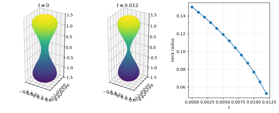
初始曲面取拉长的细颈哑铃面: 把单位球面网格的点 \((x,y,z)\) 映射为 \((s(z)x,\ s(z)y,\ 1.5z)\), 其中 \(s(z)=0.15+1.1z^2\), 得到颈部半径 \(0.15\) 的哑铃. 细颈近似半径为 \(\rho\) 的圆柱: 环向主曲率 \(-1/\rho\) 远强于轴向主曲率, 颈部近似按 \(\rho'=-1/\rho\) 收缩并在有限时间掐断, 而两端球状部分收缩慢得多——这与上一小节的二维曲线形成对比. 下面演化到掐断前停止, 记录颈部半径 (\(|z|<0.15\) 范围内顶点到 \(z\) 轴的最小距离, 各进程先取局部最小再用 allreduce 归约, 因而并行时结果不变), 并检验表面积单调下降.
The BGN scheme applies verbatim to closed surfaces in \(\mathbb R^3\): \(\kappa\) is now the mean curvature (the sum of the two principal curvatures), and a sphere satisfies \(R(t)^2=R(0)^2-4t\). Since evolve_mcf is written in a dimension-independent way, it can be used directly on surface meshes.
The initial surface is an elongated thin-neck dumbbell: each point \((x,y,z)\) of a unit-sphere mesh is mapped to \((s(z)x,\ s(z)y,\ 1.5z)\) with \(s(z)=0.15+1.1z^2\), giving a dumbbell with neck radius \(0.15\). The thin neck is approximately a cylinder of radius \(\rho\): its azimuthal principal curvature \(-1/\rho\) is far stronger than the axial one, so the neck shrinks approximately as \(\rho'=-1/\rho\) and pinches off in finite time, while the two sphere-like ends shrink much more slowly—in contrast with the planar curve of the previous subsection. Below we stop before pinch-off, record the neck radius (the minimum distance from the \(z\)-axis among vertices with \(|z|<0.15\), computed as a local minimum followed by an allreduce so that the result is unchanged in parallel), and check that the surface area decreases monotonically.
mesh_surface = UnitIcosahedralSphereMesh(refinement_level=4)
points = mesh_surface.coordinates.dat.data_ro.copy()
scale = 0.15 + 1.1*points[:, 2]**2
mesh_surface.coordinates.dat.data[:, 0] = scale*points[:, 0]
mesh_surface.coordinates.dat.data[:, 1] = scale*points[:, 1]
mesh_surface.coordinates.dat.data[:, 2] = 1.5*points[:, 2]
mesh_surface.init_cell_orientations(SpatialCoordinate(mesh_surface))

surface_step = 2.5e-4
surface_steps = 48
result_surface = evolve_mcf(
    mesh_surface, surface_step, surface_steps,
    snapshot_steps=tuple(range(4, surface_steps+1, 4)),
)

def neck_radius(coordinates, band=0.15):
    points = coordinates.dat.data_ro
    mask = np.abs(points[:, 2]) < band
    local_min = (np.linalg.norm(points[mask, :2], axis=1).min()
                 if mask.any() else np.inf)
    return coordinates.comm.allreduce(local_min, MPI.MIN)

neck_times = np.asarray(sorted(result_surface['snapshots']))
neck_radii = np.asarray([
    neck_radius(result_surface['snapshots'][t]) for t in neck_times
])
print(f'neck radius: initial = {neck_radii[0]:.4f}, '
      f'final = {neck_radii[-1]:.4f}')
print(f"surface area: initial = {result_surface['measures'][0]:.4f}, "
      f"final = {result_surface['measures'][-1]:.4f}")
assert np.all(np.diff(result_surface['measures']) < 0)
assert np.all(np.diff(neck_radii) < 0) and neck_radii[-1] < 0.06
neck radius: initial = 0.1500, final = 0.0529
surface area: initial = 7.4942, final = 6.0264
左、中图为初始与 \(t=0.012\) 时的曲面: 两端形状变化不大, 颈部明显变细. 右图中颈部半径加速下降, 实测中由 \(0.15\) 降到约 \(0.053\), 表明流动正在接近掐颈奇性; 表面积单调下降. 若继续演化, 颈部将在 \(t\approx0.013\) 附近掐断, 网格随之退化: 参数化方法无法跨越拓扑变化, 需要重新网格化, 或改用水平集等隐式描述.
The left and middle plots show the surface initially and at \(t=0.012\): the two ends barely change shape, while the neck becomes markedly thinner. The neck radius in the right plot decreases at an accelerating rate, from \(0.15\) to about \(0.053\) in our tests, indicating that the flow is approaching the pinch-off singularity; the surface area decreases monotonically. If the evolution were continued, the neck would pinch off near \(t\approx0.013\) and the mesh would degenerate: a parametric method cannot pass through the topological change, which requires remeshing or an implicit description such as a level-set method.
triangles = mesh_surface.coordinates.function_space().cell_node_map().values
fig = plt.figure(figsize=(9.5, 3.8), constrained_layout=True)
for i, t in enumerate((0.0, surface_steps*surface_step)):
    points = result_surface['snapshots'][t].dat.data_ro
    ax = fig.add_subplot(1, 3, i+1, projection='3d')
    ax.plot_trisurf(points[:, 0], points[:, 1], points[:, 2],
                    triangles=triangles, cmap='viridis', linewidth=0.1)
    ax.set_title(f'$t={t:g}$')
    ax.set_box_aspect((1, 1, 2.5))
    ax.set_xlim(-0.6, 0.6)
    ax.set_ylim(-0.6, 0.6)
    ax.set_zlim(-1.5, 1.5)
ax = fig.add_subplot(1, 3, 3)
ax.plot(neck_times, neck_radii, 'o-')
ax.set_xlabel('$t$')
ax.set_ylabel('neck radius')
_ = ax.grid(alpha=0.3)
References
John W. Barrett, Harald Garcke, and Robert Nürnberg. On the variational approximation of combined second and fourth order geometric evolution equations. SIAM Journal on Scientific Computing, 29(3):1006–1041, 2007. doi:10.1137/060653974.
Michael E. Gage and Richard S. Hamilton. The heat equation shrinking convex plane curves. Journal of Differential Geometry, 23(1):69–96, 1986. doi:10.4310/jdg/1214439902.
Matthew A. Grayson. The heat equation shrinks embedded plane curves to round points. Journal of Differential Geometry, 26(2):285–314, 1987. doi:10.4310/jdg/1214441371.