1. 并行计算 Parallel Computing#
本章内容
介绍 Firedrake 如何通过 MPI 进行并行计算: 用 mpiexec 运行脚本, 在 Jupyter 中通过 ipyparallel 执行并行代码并对照串行与并行的行为差异, 以及并行编程的常见陷阱. 部分单元需要额外安装 ipyparallel (pip install ipyparallel).
Overview
How Firedrake computes in parallel with MPI: running scripts with mpiexec, running parallel code inside Jupyter via ipyparallel while comparing serial and parallel execution, and common pitfalls of parallel programming. Some cells need the ipyparallel package (pip install ipyparallel).
1.1. Firedrake 中并行计算简介 Parallel computing in Firedrake#
Firedrake 使用 MPI 实现分布式内存并行, 并采用单程序多数据 (SPMD, single program, multiple data) 模式: 所有进程运行同一份程序, 但分别处理全局问题的不同部分.
在并行计算中, Firedrake 借助 PETSc 的 DMPlex 表示和管理网格. 网格会被划分为若干子区域并分配给不同进程; 每个进程主要存储和计算本地网格、自由度以及矩阵和向量中由自己负责的部分. 为完成分区边界附近的计算, 进程还会保存必要的 halo (或 ghost) 数据. 不同进程共享的数据通过 MPI 通信进行更新和同步.
这些并行细节大多由 Firedrake 和 PETSc 自动处理. 因此, 同一份 Firedrake 程序通常既可以串行运行, 也可以通过 MPI 启动多个进程并行运行, 而无须修改有限元问题的主体代码.
需要特别注意的是, 每个进程都会执行整份 Python 程序. 因此, 普通的 print 会被每个进程分别执行, 可能产生重复输出; 直接使用常规绘图库或自行读写文件时, 也可能出现重复操作或文件冲突. 这类与输入输出有关的操作通常需要显式指定由某个进程执行, 或者使用 Firedrake、PETSc 提供的并行安全接口.
Firedrake uses MPI for distributed-memory parallelism, following the single program, multiple data (SPMD) model: every process runs the same program, but each of them works on a different part of the global problem.
In parallel, Firedrake relies on PETSc’s DMPlex to represent and manage the mesh. The mesh is partitioned into subregions that are assigned to the processes; each process mainly stores and computes the local mesh, the degrees of freedom, and the parts of the matrices and vectors it is responsible for. In order to complete the computation near the partition boundaries, a process also keeps the necessary halo (or ghost) data. Data shared between processes is updated and synchronized through MPI communication.
Most of these parallel details are handled automatically by Firedrake and PETSc. The same Firedrake program can therefore usually be run either serially or in parallel with several MPI processes, without modifying the main body of the finite element problem.
One point deserves particular attention: every process executes the whole Python
program. An ordinary print is therefore executed by every process and may
produce duplicated output; using an ordinary plotting library, or reading and
writing files by hand, may likewise lead to duplicated operations or to file
conflicts. Such input/output operations usually have to be assigned explicitly to
one process, or to be performed through the parallel-safe interfaces provided by
Firedrake and PETSc.
1.1.1. 并行启动程序 Launching a parallel run#
Firedrake 启动并行计算只需在终端中运行以下命令:
Launching a parallel Firedrake computation only requires running the following command in a terminal:
mpiexec -n <number-of-processes> python3 /path/to/your/script.py
下面以求解 Poisson 方程的脚本 py/poisson.py 为例, 其完整内容如下:
As an example we take the script py/poisson.py, which solves the Poisson equation; its full content is:
"""并行求解 Poisson 方程的最小示例.

在 firedrake 目录下运行:

    mpiexec -n 2 python3 py/poisson.py
"""
from firedrake import *
from firedrake.petsc import PETSc

N = 4
test_mesh = RectangleMesh(N, N, 1, 1)
x, y = SpatialCoordinate(test_mesh)
f = sin(pi*x)*sin(pi*y)
g = Constant(0)

V = FunctionSpace(test_mesh, 'CG', degree=1)

u, v = TrialFunction(V), TestFunction(V)
a = inner(grad(u), grad(v))*dx
L = inner(f, v)*dx

bc = DirichletBC(V, g=g, sub_domain='on_boundary')

u_h = Function(V, name='u_h')
solve(a == L, u_h, bcs=bc)

# assemble 是集合操作, 所有进程一起调用; Print 只由 0 号进程输出
PETSc.Sys.Print(f'[{COMM_WORLD.size} process(es)] integral of u_h: '
                f'{assemble(u_h*dx):.10e}')

output = VTKFile('data/result.pvd')
output.write(u_h)
若使用 2 个进程进行计算, 在激活了 Firedrake 环境的终端中,
切换到本笔记本所在的 firedrake 目录后运行:
To run it with 2 processes, open a terminal in which the Firedrake environment is
activated, change to the firedrake directory that contains this notebook, and
run:
mpiexec -n 2 python3 py/poisson.py
脚本会先打印 u_h 的积分值 (串行与并行运行得到的值在打印的精度内相同, 更细致的比较见
如何验证并行结果是对的 How to check that a parallel result is correct), 再把解保存到 data/result.pvd.
在 data 目录下会生成一个 result 文件夹, 计算结果保存在该文件夹中, 每个进程对应一个结果文件
(2 个进程时为 result_0_0.vtu 和 result_0_1.vtu). 索引是两级的: result.pvd 指向
result/result_0.pvtu, 后者才列出各进程的 .vtu 文件; 用 ParaView 打开 result.pvd 即可,
不必关心这两级的细节.
如本节开头所述, 每个进程只负责整体网格的一个子区域, 因此每个进程的结果文件仅包含该进程对应区域的结果.
The script first prints the integral of u_h (the values obtained from a serial
and from a parallel run agree to the precision printed; see
如何验证并行结果是对的 How to check that a parallel result is correct for a finer comparison), and then saves the solution to
data/result.pvd. A result folder is created under data, and the results are
stored in it with one file per process (result_0_0.vtu and result_0_1.vtu for
2 processes). The index has two levels: result.pvd points to
result/result_0.pvtu, which in turn lists the .vtu files of the individual
processes; opening result.pvd in ParaView is all that is needed, and the two
levels can be ignored.
As said at the beginning of this section, every process is responsible for only one subregion of the whole mesh, so the result file of a process contains only the results on the corresponding subregion.
1.1.2. 输出与进程控制 Output and process control#
1.1.2.1. 并行时的输出 Output in parallel#
参考 See py/intro_utils.py
第一个进程输出 (其他进程的调用会被忽略) output from the first process only (the calls on the other processes are ignored)
PETSc.Sys.Print("This is the message will only show once!")
多个进程同步输出 synchronized output from several processes
rank, size = COMM_WORLD.rank, COMM_WORLD.size
PETSc.Sys.syncPrint(f"[{rank}/{size}] This is the message from rank {rank}!")
if rank == 0:
     PETSc.Sys.syncPrint(f"[{rank}/{size}] Message from rank {rank}!")
PETSc.Sys.syncFlush()
1.1.2.2. 仅在指定进程上运算 Computing on selected processes only#
有些事情只需要做一次, 例如打印汇总信息、写日志文件. 可以用条件语句让它们只在某个进程 (通常是 0 号进程) 上执行:
Some things only need to be done once, printing summary information or writing a log file for instance. A conditional statement can make them run on one process only, usually process 0:
u_int = assemble(u_h*dx)                  # 集合操作: 所有进程一起调用
if COMM_WORLD.rank == 0:
    print(f'integral of u_h: {u_int}')    # 纯本地操作: 可以只在 0 号进程执行
要特别小心的是, 只有纯本地操作 (普通 print、写文本文件、对已经算好的数值做后处理等) 才能放进这样的条件分支; 凡是涉及 MPI 集合通信的操作 (如 assemble、solve、norm, 甚至 triplot 绘图) 都必须所有进程一起调用, 只让部分进程执行会使程序永久挂起, 详见 并行常见陷阱 Common parallel pitfalls.
Particular care is needed here: only purely local operations (an ordinary
print, writing a text file, post-processing values that have already been
computed, and so on) may be placed inside such a branch; every operation that
involves MPI collective communication (assemble, solve, norm, or even the
plotting function triplot) must be called by all processes together, and
letting only some of them execute it makes the program hang forever, see
并行常见陷阱 Common parallel pitfalls.
1.2. 在 Jupyter 中执行并行代码 Running parallel code in Jupyter#
在 Jupyter 交互环境中, 我们可以方便地对串行代码进行测试, 从而进行快速验证.
为了在 Jupyter 环境下运行并行程序, ipyparallel 包提供了强大的支持,
它能够帮助我们在 Jupyter 中验证并行代码, 同时加深我们对 Firedrake 并行机制的理解.
In an interactive Jupyter environment serial code can be tested conveniently and
verified quickly. For running parallel programs under Jupyter, the ipyparallel
package offers strong support: it lets us validate parallel code inside Jupyter
and at the same time deepens our understanding of Firedrake’s parallel
machinery.
1.2.1. ipyparallel 简介 Introducing ipyparallel#
ipyparallel 的工作方式是: 在 notebook 之外另行启动若干独立的 Python 进程 (称为引擎, engine), notebook 通过一个客户端 (client) 把代码发送到这些引擎上执行, 再把结果取回显示. 引擎才是真正做计算的进程, notebook 自身的内核仍然是单进程的.
下面创建并连接一个包含 2 个引擎的集群: engines="mpi" 表示用 MPI 启动引擎, 使这 2 个引擎构成一个 MPI 通信组 (效果相当于 mpiexec -n 2), Firedrake 在其中即可按前面介绍的方式并行计算; start_and_connect_sync() 启动集群并等待所有引擎就绪, 返回与之通信的客户端.
ipyparallel works as follows: a number of separate Python processes (called
engines) are started outside the notebook, the notebook sends code to these
engines through a client, and fetches the results back for display. The engines
are the processes that actually compute; the kernel of the notebook itself
remains a single process.
The following creates and connects to a cluster of 2 engines: engines="mpi"
means that the engines are launched through MPI, so that these 2 engines form one
MPI communication group (the effect is that of mpiexec -n 2), in which
Firedrake can compute in parallel in the way described above;
start_and_connect_sync() starts the cluster, waits for all engines to be ready,
and returns the client that talks to them.
Tip
这里必须写 engines="mpi". 若改用 ipp.Cluster(profile="mpi"), 在本机缺少相应 profile 时会静默退化为若干互不通信的单进程引擎 (每个引擎中 COMM_WORLD 的大小都是 1), 看起来能运行, 但并没有真正并行.
Tip
engines="mpi" is essential here. With ipp.Cluster(profile="mpi") instead, a
machine that lacks the corresponding profile silently falls back to several
single-process engines that do not communicate with each other (COMM_WORLD has
size 1 in every engine); it looks as if it runs, but there is no real
parallelism.
import ipyparallel as ipp

cluster = ipp.Cluster(engines="mpi", n=2)
client = cluster.start_and_connect_sync()
集群就绪后, 用 ipyparallel 提供的魔法指令 %%px 可以把整个单元的代码发送到所有引擎上同时执行. --block 表示同步执行: 等所有引擎都运行完毕后再继续执行后面的单元, 这样输出更便于对照.
Once the cluster is ready, the magic %%px provided by ipyparallel sends the
code of a whole cell to all engines to be executed simultaneously. --block
means synchronous execution: the following cells are only executed after all
engines have finished, which makes the output easier to compare.
1.2.2. 执行并行代码 Running parallel code#
下面的单元在 2 个引擎上分别导入 Firedrake 并生成网格, 然后打印各自的进程编号和总进程数: mesh.comm 是该网格所在的 MPI 通信子, 由它取得的 size 为 2, 说明两个引擎确实位于同一个 MPI 通信组中. 输出仍按 前面介绍的方式 控制: syncPrint 配合 syncFlush 按进程编号顺序输出每个进程的信息, Print 只输出一次.
The cell below imports Firedrake on the 2 engines and generates a mesh on each of
them, then prints their own rank and the total number of processes: mesh.comm
is the MPI communicator the mesh lives on, and the size obtained from it is 2,
which shows that the two engines really do belong to the same MPI communication
group. The output is still controlled as introduced above:
syncPrint together with syncFlush prints the message of every process in rank
order, while Print prints only once.
%%px --block
from firedrake import *
from firedrake.petsc import PETSc

N = 4
mesh = RectangleMesh(N, N, 1, 1)

rank, size = mesh.comm.rank, mesh.comm.size
PETSc.Sys.syncPrint(f"[{rank}/{size}] This is the message from rank {rank}!")
PETSc.Sys.syncFlush()

PETSc.Sys.Print(f"[{rank}/{size}] This message only from rank 0!")
[stdout:0] [0/2] This is the message from rank 0!
[1/2] This is the message from rank 1!
[0/2] This message only from rank 0!
提示: 输出中的 [stdout:0] 前缀 Tip: the [stdout:0] prefix in the output
%%px 显示多个引擎的输出时, 会为每个引擎加上 [stdout:<引擎编号>] 前缀. 该前缀由 ipyparallel 在内部硬编码 (见 AsyncResult.display_outputs), 没有提供修改文本的配置项; %%px 只能用 --group-outputs 改变分组顺序, 或用 -t/--targets 限制参与执行的引擎. 另外, 连续来自同一引擎的多行输出只在开头显示一次前缀.
上面的例子中所有信息都由 0 号引擎打印, 因此只出现一个 [stdout:0]: PETSc.Sys.syncPrint 把各进程的消息汇总到 0 号进程, 再由 syncFlush 一次输出, 各行开头的 [rank/size] 是我们自己加的进程标识. 需要区分进程时, 这种写法比依赖 ipyparallel 的前缀更可控.
若想完全自定义显示方式, 可以不用 %%px 的自动显示, 而是直接处理执行结果:
When %%px displays the output of several engines, it prefixes the output of
each engine with [stdout:<engine id>]. This prefix is hard-coded inside
ipyparallel (see AsyncResult.display_outputs) and there is no configuration
option to change its text; %%px can only change the grouping order with
--group-outputs, or restrict the engines taking part in the execution with
-t/--targets. Moreover, consecutive lines of output from the same engine only
carry the prefix once, at the beginning.
In the example above all the messages are printed by engine 0, so only one
[stdout:0] appears: PETSc.Sys.syncPrint gathers the messages of all processes
on process 0, which syncFlush then prints in one go, and the [rank/size] at
the beginning of each line is a process label we added ourselves. When
processes have to be told apart, this is more controllable than relying on ipyparallel’s prefix.
For a completely custom display, the automatic display of %%px can be avoided
and the execution result processed directly:
ar = client[:].execute(
    "from mpi4py import MPI; print(f'rank {MPI.COMM_WORLD.rank}')", block=True
)
for eid, out in zip(ar.engine_id, ar.stdout):
    for line in out.rstrip('\n').split('\n'):
        print(f'<engine {eid}> {line}')
输出为:
The output is:
<engine 0> rank 0
<engine 1> rank 1
1.2.3. %%px 的更多用法 More about %%px#
前面用的一直是最简单的 %%px --block, 它把整个单元发给所有引擎并等待全部完成. 这里补充几个常用的参数.
-t/--targets 用来只让部分引擎执行, 例如 --targets 0 表示只在 0 号引擎上运行. 下面用它打印引擎的工作目录:
So far we have only used the simplest form %%px --block, which sends the whole
cell to all engines and waits for all of them to finish. A few more commonly
used options are added here.
-t/--targets restricts the execution to some of the engines; --targets 0,
for example, runs on engine 0 only. We use it below to print the working
directory of an engine:
%%px --block --targets 0
import os
print(f'cwd basename            : {os.path.basename(os.getcwd())}')
print(f'py/intro_utils.py exists: {os.path.exists("py/intro_utils.py")}')
[stdout:0] cwd basename            : firedrake
py/intro_utils.py exists: True
两行输出合起来说明: 引擎当前目录的名字就是 firedrake, 而且在这个目录下用相对路径 py/intro_utils.py 确实找得到文件. 也就是说, 引擎的工作目录是启动本 notebook 的那个目录, 而不是引擎自己的某个临时目录. 这一点很容易被忽略, 却是本章能跑通的前提: 后面并行单元里的 from py.intro_utils import triplot 之所以在引擎里也能成功, 靠的正是这一点; 换个目录启动 notebook, 同样的代码就会在引擎里抛出 ModuleNotFoundError. 引擎里用相对路径读写文件同理, 例如 并行下的 I/O 一节用 CheckpointFile 写出的 data/parallel_checkpoint.h5, 也落在这个目录下.
要提醒的是, --targets 只适合放纯本地的操作. 单元里一旦出现集合操作 (assemble、solve、norm 等), 只让部分引擎执行就会挂起, 原因见 并行常见陷阱 Common parallel pitfalls.
Taken together, the two lines of output show that the name of the engine’s
current directory is firedrake, and that the relative path
py/intro_utils.py really does find a file in that directory. In other words,
the working directory of the engines is the directory from which this notebook
was started, and not some temporary directory of their own. This is easily
overlooked, yet it is the precondition for this chapter to run at all: the
from py.intro_utils import triplot in the parallel cells below succeeds inside
the engines precisely because of it, and starting the notebook from another
directory would make the same code raise ModuleNotFoundError in the engines.
The same applies to relative paths used for reading and writing files in the
engines; the data/parallel_checkpoint.h5 written with CheckpointFile in the
section on I/O in parallel, for example, also ends up
in this directory.
It should be pointed out that --targets is only suitable for purely local
operations. As soon as a cell contains a collective operation (assemble,
solve, norm, …), letting only some of the engines execute it makes the
program hang; the reason is given in 并行常见陷阱 Common parallel pitfalls.
--noblock 则相反: 把代码发出去就立刻返回, 不等引擎算完, 单元的值是一个 AsyncResult 对象. 这样可以在引擎慢慢算的同时, 继续在本地内核里做别的事. 稍后用 %pxresult 取回并显示上一次异步执行的输出:
--noblock does the opposite: it sends the code off and returns immediately
without waiting for the engines to finish, and the value of the cell is an
AsyncResult object. This makes it possible to carry on with other work in the
local kernel while the engines are computing. The output of the last asynchronous
execution is fetched and displayed later with %pxresult:
%%px --noblock
import time
time.sleep(1)
slow_value = 'the slow cell has finished'
PETSc.Sys.Print(slow_value)
<AsyncResult(%px): pending>
%pxresult
[stdout:0]
the slow cell has finished
--noblock 那个单元立刻返回了一个 <AsyncResult(%px): pending>, 说明它没有等待; 直到执行 %pxresult, 才阻塞着等引擎算完并显示输出. 若想在代码里显式等待, 可以把 AsyncResult 存到变量里再等它: %%px --noblock --out ar, 然后在后面的单元中调用 ar.wait().
另外还有 %autopx: 打开之后每一个单元都会自动发到引擎上执行, 直到再次执行 %autopx 关闭. 它省去了反复写 %%px, 但也很容易忘记关闭, 使本该在本地运行的单元跑到引擎上去, 因此本章没有使用它.
最后再强调一次: 引擎和本地内核是不同的进程, 变量互不相通. 要把本地的值送到引擎上, 用 client[:].push({'name': value}); 要把引擎上的结果取回本地, 用 client[0].pull('name', block=True) —— 后者在后面比较串行与并行结果时会实际用到.
The cell with --noblock returned a <AsyncResult(%px): pending> immediately,
which shows that it did not wait; only %pxresult blocks until the engines have
finished and then displays the output. To wait explicitly in code, the
AsyncResult can be stored in a variable with %%px --noblock --out ar and
waited for with ar.wait() in a later cell.
There is also %autopx: once it is switched on, every cell is automatically
sent to the engines, until %autopx is executed again to switch it off. It saves
writing %%px over and over, but it is also easily forgotten, which sends cells
that were meant to run locally to the engines; this chapter therefore does not
use it.
One last reminder: the engines and the local kernel are different processes, and
their variables are separate. To send a local value to the engines, use
client[:].push({'name': value}); to fetch a result from the engines back to the
local kernel, use client[0].pull('name', block=True) — the latter is actually
used below when serial and parallel results are compared.
1.3. 使用 ipyparallel 观察串行和并行过程 Observing serial and parallel execution with ipyparallel#
下面每个小节都用几乎相同的代码运行两遍: 不加 %%px 的单元在 notebook 自身的本地内核 (单进程) 中运行, 加了 %%px --block 的单元则发送到前面启动的集群引擎上运行. 两边各自维护自己的一套变量, 互不干扰: 后续不带 %%px 的单元使用的是本地内核里最近一次定义的 mesh/V1/V2/W 等对象, 带 %%px 的单元使用的则是集群引擎里最近一次通过 %%px 定义的同名对象. 通过对照两侧的输出, 可以直观看到同一段 Firedrake 代码在串行和并行下的行为差异.
为便于区分, 下文每个代码单元前都有一行粗体标注: 串行 (本地内核) 表示该单元在本地内核中运行, 并行 (2 个引擎) 表示该单元以 %%px --block 开头、在集群引擎上运行; 当并行单元的代码与其串行版本完全相同 (仅首行多出 %%px --block) 时, 默认折叠并行单元的代码, 需要时点击展开查看.
Each of the following subsections runs almost the same code twice: the cell
without %%px runs in the notebook’s own local kernel (a single process), while
the cell with %%px --block is sent to the cluster engines started above. The
two sides maintain their own sets of variables and do not interfere with each
other: a later cell without %%px uses the mesh/V1/V2/W objects most
recently defined in the local kernel, whereas a cell with %%px uses the objects
of the same names most recently defined through %%px in the cluster engines.
Comparing the outputs of the two sides shows directly how the same piece of
Firedrake code behaves in serial and in parallel.
To tell them apart, every code cell below is preceded by a bold label:
Serial (local kernel) means that the cell runs in the local kernel, and
Parallel (2 engines) means that the cell starts with %%px --block and runs on the
cluster engines. When the code of a parallel cell is identical to its serial
version (apart from the extra first line %%px --block), the parallel cell is
collapsed by default; click to expand it when needed.
1.3.1. 生成网格并画出网格 Generating and plotting the mesh#
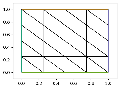
串行 (本地内核): 先在本地内核里生成 4×4 网格并画出, 作为对照基准; mesh.topology_dm.view() 输出该网格对应 DMPlex 的拓扑信息.
Serial (local kernel): a 4×4 mesh is first generated and plotted in the local kernel,
as the reference; mesh.topology_dm.view() prints the topology information of
the DMPlex corresponding to this mesh.
from firedrake import *
from py.intro_utils import triplot
from firedrake.petsc import PETSc

import matplotlib.pyplot as plt

N = 4
mesh = RectangleMesh(N, N, 1, 1)
mesh.topology_dm.view()
fig, axes = plt.subplots(figsize=[4, 3])
triplot(mesh, axes=axes)
axes.set_xlim([-0.1, 1.1])
axes.set_ylim([-0.1, 1.1])
fig.tight_layout()
DM Object: DM_0x2983a2b0_0 1 MPI process
  type: plex
DM_0x2983a2b0_0 in 2 dimensions:
  Number of 0-cells per rank: 25
  Number of 1-cells per rank: 56
  Number of 2-cells per rank: 32
Labels:
  celltype: 3 strata with value/size (0 (25), 1 (56), 3 (32))
  depth: 3 strata with value/size (0 (25), 1 (56), 2 (32))
  marker: 1 strata with value/size (1 (32))
  Face Sets: 4 strata with value/size (1 (9), 2 (9), 3 (9), 4 (9))
  exterior_facets: 1 strata with value/size (1 (32))
  interior_facets: 1 strata with value/size (1 (63))
  pyop2_core: 1 strata with value/size (1 (113))
  pyop2_owned: 0 strata with value/size ()
  pyop2_ghost: 0 strata with value/size ()
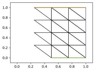
并行 (2 个引擎): 在集群的 2 个引擎上重复相同代码; mesh.comm 此时是各引擎自己的 MPI 通信子, 生成的网格会被 DMPlex 自动划分到 2 个进程.
Parallel (2 engines): the same code is repeated on the 2 engines of the cluster;
mesh.comm is now each engine’s own MPI communicator, and the mesh generated is
automatically partitioned by DMPlex over the 2 processes.
[stdout:0] DM Object: DM_0x90cb510_1 2 MPI processes
  type: plex
DM_0x90cb510_1 in 2 dimensions:
  Number of 0-cells per rank: 19 19
  Number of 1-cells per rank: 38 38
  Number of 2-cells per rank: 20 20
Labels:
  depth: 3 strata with value/size (0 (19), 1 (38), 2 (20))
  celltype: 3 strata with value/size (0 (19), 1 (38), 3 (20))
  marker: 1 strata with value/size (1 (19))
  Face Sets: 3 strata with value/size (2 (9), 3 (5), 4 (7))
  exterior_facets: 1 strata with value/size (1 (19))
  interior_facets: 1 strata with value/size (1 (47))
  pyop2_core: 1 strata with value/size (1 (26))
  pyop2_owned: 1 strata with value/size (1 (26))
  pyop2_ghost: 1 strata with value/size (1 (25))
[output:0]
[output:1]
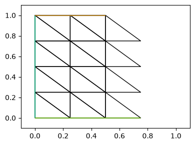
可以看到上面并行中两个网格图分别只是整体网格的一部分, 且边界处有重叠 (ghost/halo 单元): 这些重叠单元使每个进程在组装局部矩阵时也能访问到相邻单元的信息.
两段 mesh.topology_dm.view() 输出中的数字也值得对照:
串行时网格共有 25 个顶点 (0-cells)、56 条边 (1-cells)、32 个单元 (2-cells); 并行时每个进程各有 19 个顶点、38 条边、20 个单元. 注意 20 + 20 = 40 > 32: 多出的 8 个单元正是分区边界两侧互相重叠的 ghost 单元, 顶点和边同理.
pyop2_core、pyop2_owned、pyop2_ghost把 DMPlex 的点 (顶点、边、单元的统称) 分为三类 (含义见 后文): 串行时全部 113 = 25 + 56 + 32 个点都是 core; 并行时 0 号进程为 26、26、25, 三者之和 77 = 19 + 38 + 20.Labels一段只显示 0 号进程的信息, 并行输出中Face Sets只列出 2、3、4 三个值: 编号为 1 的那条边界完全落在 1 号进程上, 0 号进程没有它的任何一段. 这正是本章从 py/intro_utils.py 导入triplot包装函数的原因: 并行绘图时, 拿不到某条边界的进程会收到 Firedrake 的 “Subdomain is empty” 警告, 包装函数把这条无害的警告过滤掉了.
The two mesh plots produced in parallel above are each only a part of the whole mesh, and they overlap near the partition boundary (the ghost/halo cells): these overlapping cells let every process access the information of its neighboring cells when it assembles the local matrix.
The numbers in the two mesh.topology_dm.view() outputs are worth comparing as
well:
In serial the mesh has 25 vertices (0-cells), 56 edges (1-cells) and 32 cells (2-cells); in parallel each process has 19 vertices, 38 edges and 20 cells. Note that 20 + 20 = 40 > 32: the 8 extra cells are exactly the ghost cells that overlap on both sides of the partition boundary, and the same holds for the vertices and the edges.
pyop2_core,pyop2_ownedandpyop2_ghostdivide the points of the DMPlex (the common name for vertices, edges and cells) into three classes (their meaning is explained later on): in serial all 113 = 25 + 56 + 32 points are core; in parallel process 0 has 26, 26 and 25, whose sum is 77 = 19 + 38 + 20.The
Labelspart only shows the information of process 0, and in the parallel outputFace Setslists only the three values 2, 3 and 4: the boundary numbered 1 lies entirely on process 1, and process 0 holds no part of it. This is exactly why this chapter imports thetriplotwrapper from py/intro_utils.py: when plotting in parallel, a process that holds no part of some boundary receives Firedrake’s “Subdomain is empty” warning, and the wrapper filters this harmless warning out.
1.3.2. 分区重叠 (overlap) 的显式控制 Explicit control of the partition overlap#
上面看到的 ghost 单元并不是固定不变的, 它由建网格时的 distribution_parameters 控制. 其中 overlap_type 是一个二元组 (类型, 层数): Firedrake 的默认值是 (DistributedMeshOverlapType.FACET, 1), 表示每个进程除了自己拥有的单元, 再多保留一层”与本进程单元共享一条边 (面) 的邻居单元”; 改成 (DistributedMeshOverlapType.NONE, 0) 就完全关闭重叠, 改成 (DistributedMeshOverlapType.FACET, 2) 则保留两层.
下面用同一个 4×4 网格把三种设置各建一次, 只看单元的计数: cell_set.size 是本进程拥有的单元数, cell_set.total_size 还包含 ghost 单元, 两者之差就是 ghost 单元数 (这个三段划分的含义见 后文). 注意这里用的是新变量名 mesh_ovlp, 后面各小节继续使用的仍是前面生成的 mesh. 单元开头之所以还要重新取一次 rank 和 size, 原因见 from firedrake import * 会覆盖 rank 等变量 from firedrake import * overwrites variables such as rank.
The ghost cells seen above are not fixed; they are controlled by
distribution_parameters when the mesh is built. Its overlap_type is a pair (type, number of layers): the Firedrake default is
(DistributedMeshOverlapType.FACET, 1), meaning that besides the cells it owns,
each process keeps one further layer of “neighboring cells that share an edge
(facet) with a cell of this process”; (DistributedMeshOverlapType.NONE, 0)
switches the overlap off completely, and (DistributedMeshOverlapType.FACET, 2)
keeps two layers.
Below the same 4×4 mesh is built once for each of the three settings, and only
the cell counts are looked at: cell_set.size is the number of cells owned by
this process and cell_set.total_size also includes the ghost cells, so the
difference of the two is the number of ghost cells (the meaning of this
three-way split is explained later on). Note that a
new variable name mesh_ovlp is used here; the later subsections keep using the
mesh generated before. The reason why rank and size are fetched once more
at the beginning of the cell is explained in from firedrake import * 会覆盖 rank 等变量 from firedrake import * overwrites variables such as rank.
并行 (2 个引擎) Parallel (2 engines)
%%px --block
rank, size = mesh.comm.rank, mesh.comm.size   # 重新取一次: firedrake 也导出了名为 rank 的函数
for label, overlap in (('(NONE, 0) ', (DistributedMeshOverlapType.NONE, 0)),
                       ('(FACET, 1)', (DistributedMeshOverlapType.FACET, 1)),
                       ('(FACET, 2)', (DistributedMeshOverlapType.FACET, 2))):
    mesh_ovlp = RectangleMesh(N, N, 1, 1,
                              distribution_parameters={'overlap_type': overlap})
    cells = mesh_ovlp.cell_set
    PETSc.Sys.syncPrint(f'[{rank}/{size}] overlap_type={label} '
                        f'owned cells: {cells.size:>3}, '
                        f'total cells: {cells.total_size:>3}, '
                        f'ghost cells: {cells.total_size - cells.size:>3}')
    PETSc.Sys.syncFlush()
[stdout:0] [0/2] overlap_type=(NONE, 0)  owned cells:  16, total cells:  16, ghost cells:   0
[1/2] overlap_type=(NONE, 0)  owned cells:  16, total cells:  16, ghost cells:   0
[0/2] overlap_type=(FACET, 1) owned cells:  16, total cells:  20, ghost cells:   4
[1/2] overlap_type=(FACET, 1) owned cells:  16, total cells:  20, ghost cells:   4
[0/2] overlap_type=(FACET, 2) owned cells:  16, total cells:  24, ghost cells:   8
[1/2] overlap_type=(FACET, 2) owned cells:  16, total cells:  24, ghost cells:   8
对照三行输出可以看到: owned cells 一列始终是 16, 变化的是 total cells —— 关掉重叠后它从 20 变回 16, ghost 单元为 0. 这正是 overlap 的含义: 它只增加每个进程本地存储的单元数, 不改变每个进程真正拥有的单元数. 而 16 + 16 = 32 恰是整张网格的单元总数, 上一段”20 + 20 = 40 > 32, 多出的 8 个是 ghost 单元”这句话, 到这里就变成了可以直接读出来的数字. 把层数加到 2, ghost 单元又从 4 增加到 8: 重叠层越厚, 每个进程需要额外保存和同步的数据就越多.
有两点需要说明:
这个对照只在并行下才有意义. 串行运行时整张网格都在一个进程上, 没有分区也就没有重叠, 三种设置得到的计数完全相同 (都是 32 个单元、0 个 ghost).
不要因为”关掉重叠更省内存”就随手改这个参数. 像本章这样只含单元内部积分 (
dx) 的 CG 问题, 关掉重叠后仍能算出正确结果 (实测串行与并行的积分值一致), 因为 CG 的自由度交换只依赖分区边界上的节点; 但只要计算需要用到相邻单元的数据 —— 例如间断 Galerkin 方法的内部面积分dS(见 Poisson 方程 II 的 SIPG 一节) —— 缺少重叠层就会出错, 实测甚至会让程序直接崩溃, 而不是给出清晰的报错. 默认的(FACET, 1)正是为了让这些常见用法开箱即用.
Comparing the three lines of output: the owned cells column is always 16, and
what changes is total cells — with the overlap switched off it drops from 20
back to 16 and there are no ghost cells. This is exactly what the overlap means:
it only increases the number of cells each process stores locally, and does
not change the number of cells each process really owns. And 16 + 16 = 32 is
precisely the total number of cells of the whole mesh, so the sentence of the
previous paragraph, “20 + 20 = 40 > 32, the 8 extra ones being ghost cells”,
becomes a number that can be read off directly here. Raising the number of layers
to 2 increases the ghost cells from 4 to 8: the thicker the overlap, the more
data each process has to store and to synchronize in addition.
Two remarks:
This comparison is only meaningful in parallel. In a serial run the whole mesh is on one process, there is no partitioning and hence no overlap, and the three settings give exactly the same counts (32 cells and 0 ghost cells in all three cases).
Do not change this parameter casually just because “switching the overlap off saves memory”. For a CG problem such as the one of this chapter, which only contains cell integrals (
dx), the result is still correct with the overlap switched off (in our tests the integral values in serial and in parallel agree), because the exchange of degrees of freedom for CG only depends on the nodes on the partition boundary; but as soon as the computation needs data from neighboring cells — the interior facet integraldSof a discontinuous Galerkin method, for example (see the SIPG section of Poisson equation II) — a missing overlap layer gives wrong results, and in our tests it even made the program crash outright instead of reporting a clear error. The default(FACET, 1)is there precisely to make these common use cases work out of the box.
1.3.3. 定义变分问题 Defining the variational problem#
定义一个简单的混合变分问题 (向量分量 \(u_1\) 用 \([P_1]^2\), 标量分量 \(u_2\) 用 \(P_2\)), 后续几个小节都基于这里定义的 mesh、V1、V2、W 展开.
A simple mixed variational problem is defined (the vector component \(u_1\) in
\([P_1]^2\), the scalar component \(u_2\) in \(P_2\)); the next few subsections all
build on the mesh, V1, V2 and W defined here.
串行 (本地内核) Serial (local kernel)
V1 = VectorFunctionSpace(mesh, 'CG', 1)
V2 = FunctionSpace(mesh, 'CG', 2)
W = MixedFunctionSpace([V1, V2])  # W = V1*V2
u1, u2 = TrialFunctions(W)
v1, v2 = TestFunctions(W)
a = dot(u1, v1)*dx + u2*v2*dx

x, y = SpatialCoordinate(mesh)
f = dot(as_vector((sin(x), cos(y))), v1)*dx + cos(y)*v2*dx

bc = DirichletBC(W.sub(0), 0, 1)
uh = Function(W)
problem = LinearVariationalProblem(a, f, uh, bcs=bc)
并行 (2 个引擎) Parallel (2 engines)
两段代码完全相同, 区别只在于后者由 %%px 分发到两个引擎上执行: W 在每个进程上只保存该进程负责的那部分自由度.
The two pieces of code are exactly the same; the only difference is that the
latter is distributed to the two engines by %%px: on each process W only
stores the part of the degrees of freedom that process is responsible for.
1.3.4. 函数空间维度 The dimension of a function space#
函数空间的自由度个数可以从几个角度查看, 下面以 V1 为例. V1.dim() 返回全局自由度总数, 所有进程上一致; node_count 和 dof_count 则是含 halo 的本地计数: 除了本进程拥有的节点/自由度外, 还包括从相邻进程同步来的 ghost 节点/自由度.
The number of degrees of freedom of a function space can be looked at from
several angles; V1 is taken as an example below. V1.dim() returns the total
number of global degrees of freedom and is the same on all processes;
node_count and dof_count, on the other hand, are local counts including the
halo: besides the nodes/degrees of freedom owned by this process, they also
include the ghost nodes/degrees of freedom synchronized from the neighboring
processes.
串行 (本地内核) Serial (local kernel)
rank, size = mesh.comm.rank, mesh.comm.size
PETSc.Sys.Print(f'Number of dofs of V1: {V1.dim()}')
PETSc.Sys.syncPrint(f'[{rank}/{size}] V1 Node count: {V1.node_count}; V1 Dof count: {V1.dof_count}')
PETSc.Sys.syncFlush()
Number of dofs of V1: 50
[0/1] V1 Node count: 25; V1 Dof count: 50
并行 (2 个引擎) Parallel (2 engines)
[stdout:0] Number of dofs of V1: 50
[0/2] V1 Node count: 19; V1 Dof count: 38
[1/2] V1 Node count: 19; V1 Dof count: 38
串行时 node_count 就是全局节点数 25, dof_count 是它的 2 倍 (每个节点上有 2 个分量). 并行时两个进程的 node_count 恰好都是 19, 但组成并不相同: 0 号进程是 10 个自身拥有的节点加 9 个 ghost 节点, 1 号进程是 15 个加 4 个. 拥有的节点数之和 10 + 15 = 25 恰为全局节点数; 而 19 + 19 = 38 > 25, 多出的正是分区边界两侧互为 ghost 的节点. 各进程拥有的节点数可以从后文的 node_set.size 读出.
In serial node_count is just the global number of nodes, 25, and dof_count is
twice that (each node carries 2 components). In parallel the node_count of the
two processes happens to be 19 in both cases, but they are not composed in the
same way: process 0 has 10 nodes of its own plus 9 ghost nodes, process 1 has 15
plus 4. The numbers of owned nodes add up to 10 + 15 = 25, exactly the global
number of nodes; whereas 19 + 19 = 38 > 25, the excess being the nodes on either
side of the partition boundary that are ghosts for the other process. The number
of nodes owned by each process can be read off from node_set.size below.
为进一步观察本地和 ghost 自由度的区别, 下面创建一个 Function, 分别用 PETSc Vec 的只读视图 (dat.vec_ro) 和 dat 的只读数组视图 (data_ro、data_ro_with_halos) 查看它的本地大小. 顺带一提, 只读访问数据请用 data_ro 系列属性; 可写的 data 会把 halo 标记为失效, 使下一次访问带 halo 的数据时触发同步通信.
To look more closely at the difference between local and ghost degrees of
freedom, a Function is created below and its local size is inspected through
the read-only view of the PETSc Vec (dat.vec_ro) and through the read-only
array views of dat (data_ro, data_ro_with_halos). Incidentally, read-only
access to the data should use the data_ro family of properties; the writable
data marks the halo as invalid, so that the next access to the data with halo
triggers a synchronizing communication.
串行 (本地内核) Serial (local kernel)
f_v1 = Function(V1)
with f_v1.dat.vec_ro as vec:
    PETSc.Sys.syncPrint(f'[{rank}/{size}] vec sizes: {vec.getSizes()}')
    PETSc.Sys.syncFlush()
PETSc.Sys.syncPrint(f'[{rank}/{size}] data: {f_v1.dat.data_ro.shape}, '
                    f'data_with_halos: {f_v1.dat.data_ro_with_halos.shape}')
PETSc.Sys.syncFlush()
[0/1] vec sizes: (50, 50)
[0/1] data: (25, 2), data_with_halos: (25, 2)
并行 (2 个引擎) Parallel (2 engines)
[stdout:0] [0/2] vec sizes: (20, 50)
[1/2] vec sizes: (30, 50)
[0/2] data: (10, 2), data_with_halos: (19, 2)
[1/2] data: (15, 2), data_with_halos: (19, 2)
vec.getSizes() 返回的二元组是 (本地长度, 全局长度): 串行时为 (50, 50); 并行时全局长度不变, 本地长度 20 和 30 分别是两个进程拥有的自由度数 (10 个和 15 个节点, 每个节点 2 个分量). data_ro 的形状与之对应: (10, 2) 和 (15, 2) 只含本进程拥有的自由度, 10 × 2 = 20 正是 Vec 的本地长度; data_ro_with_halos 的形状 (19, 2) 则与前面的 node_count 一致, 额外包含了 ghost 自由度. 串行时没有 ghost 区域, 两种视图大小相同.
The pair returned by vec.getSizes() is (local length, global length): (50, 50)
in serial; in parallel the global length is unchanged, and the local lengths 20
and 30 are the numbers of degrees of freedom owned by the two processes (10 and
15 nodes with 2 components each). The shapes of data_ro correspond to them:
(10, 2) and (15, 2) contain only the degrees of freedom owned by this process,
and 10 × 2 = 20 is exactly the local length of the Vec; the shape (19, 2) of
data_ro_with_halos agrees with the node_count above and contains the ghost
degrees of freedom in addition. In serial there is no halo region and the two
views have the same size.
1.3.5. 节点集和自由度数据集 Node sets and degree-of-freedom data sets#
PyOP2 用 node_set 和 dof_dset 描述一个函数空间在各进程上如何切分: node_set 对应网格节点 (自由度承载点), dof_dset 在此基础上进一步考虑每个节点上的分量数 (如向量场每个节点有多个自由度). 下面打印它们的 str 和 repr: str 中的 size 是本进程拥有的节点数, repr 中的三元组是 (core_size, size, total_size), 含义见下一小节.
PyOP2 uses node_set and dof_dset to describe how a function space is split
among the processes: node_set corresponds to the mesh nodes (the points that
carry the degrees of freedom), and dof_dset additionally takes into account the
number of components at each node (a vector field, for instance, has several
degrees of freedom per node). Their str and repr are printed below: the size
in str is the number of nodes owned by this process, and the triple in repr
is (core_size, size, total_size), whose meaning is explained in the next
subsection.
串行 (本地内核) Serial (local kernel)
PETSc.Sys.syncPrint(f'[{rank}/{size}] V1: {str(V1.node_set)}')
PETSc.Sys.syncPrint(f'[{rank}/{size}]     {repr(V1.node_set)}')
PETSc.Sys.syncPrint(f'[{rank}/{size}] V1: {str(V1.dof_dset)}')
PETSc.Sys.syncPrint(f'[{rank}/{size}]     {repr(V1.dof_dset)}')
PETSc.Sys.syncFlush()
[0/1] V1: OP2 Set: set_#x7f9057f67260 with size 25
[0/1]     Set((np.int64(25), np.int64(25), np.int64(25)), 'set_#x7f9057f67260')
[0/1] V1: OP2 DataSet: None_nodes_dset on set OP2 Set: set_#x7f9057f67260 with size 25, with dim (2,), False
[0/1]     DataSet(Set((np.int64(25), np.int64(25), np.int64(25)), 'set_#x7f9057f67260'), (2,), 'None_nodes_dset', False)
并行 (2 个引擎) Parallel (2 engines)
[stdout:0] [0/2] V1: OP2 Set: set_#x7f2995df6e40 with size 10
[0/2]     Set((np.int64(5), np.int64(10), np.int64(19)), 'set_#x7f2995df6e40')
[0/2] V1: OP2 DataSet: None_nodes_dset on set OP2 Set: set_#x7f2995df6e40 with size 10, with dim (2,), False
[0/2]     DataSet(Set((np.int64(5), np.int64(10), np.int64(19)), 'set_#x7f2995df6e40'), (2,), 'None_nodes_dset', False)
[1/2] V1: OP2 Set: set_#x7ff64da538c0 with size 15
[1/2]     Set((np.int64(10), np.int64(15), np.int64(19)), 'set_#x7ff64da538c0')
[1/2] V1: OP2 DataSet: None_nodes_dset on set OP2 Set: set_#x7ff64da538c0 with size 15, with dim (2,), False
[1/2]     DataSet(Set((np.int64(10), np.int64(15), np.int64(19)), 'set_#x7ff64da538c0'), (2,), 'None_nodes_dset', False)
1.3.5.1. Set 与 DataSet 的各种 size The various sizes of a Set and a DataSet#
参考 Reference: firedrakeproject/firedrake
Set 中的元素按下标分成三段, 段的边界由 core_size、size、total_size 三个属性给出:
[0, core_size): 本进程拥有、且计算时不依赖任何 halo 数据的元素;[core_size, size): 本进程拥有的其余元素, 它们与其他进程相邻, 计算时可能用到 halo 数据;[size, total_size): ghost 元素, 由其他进程拥有, 本进程只保存副本.
属性 sizes 即三元组 (core_size, size, total_size). 对照下面的输出: 0 号进程的 node_set 三元组为 (5, 10, 19), 即它拥有 10 个节点 (其中 5 个完全不与 ghost 节点相邻), 加上 9 个 ghost 节点后本地共存储 19 个; 串行时没有 ghost, 三个数都等于全局节点数 25.
The elements of a Set are divided by index into three ranges, whose boundaries
are given by the three attributes core_size, size and total_size:
[0, core_size): elements owned by this process whose computation does not depend on any halo data;[core_size, size): the remaining elements owned by this process; they are adjacent to other processes and their computation may use halo data;[size, total_size): ghost elements, owned by other processes, of which this process only keeps a copy.
The attribute sizes is the triple (core_size, size, total_size). Compare with
the output below: the node_set triple of process 0 is (5, 10, 19), i.e. it owns
10 nodes (5 of which are not adjacent to any ghost node) and stores 19 of them
locally once the 9 ghost nodes are added; in serial there are no ghosts and all
three numbers equal the global number of nodes, 25.
串行 (本地内核) Serial (local kernel)
node_set = V1.node_set
msg = f'core size: {node_set.core_size}, size: {node_set.size}, total size: {node_set.total_size}'
PETSc.Sys.syncPrint(f'[{rank}/{size}] {msg}')
PETSc.Sys.syncFlush()
[0/1] core size: 25, size: 25, total size: 25
并行 (2 个引擎) Parallel (2 engines)
[stdout:0] [0/2] core size: 5, size: 10, total size: 19
[1/2] core size: 10, size: 15, total size: 19
串行 (本地内核) Serial (local kernel)
dof_dset = V1.dof_dset
size_msg = f'core size: {dof_dset.core_size}, size: {dof_dset.size}, total size: {dof_dset.total_size}'
# dim: shape tuple of the values for each element, cdim: product of dim tuple
dim_msg = f'dim: {dof_dset.dim}, cdim: {dof_dset.cdim}'
PETSc.Sys.syncPrint(f'[{rank}/{size}] {size_msg}, {dim_msg}')
PETSc.Sys.syncFlush()
[0/1] core size: 25, size: 25, total size: 25, dim: (2,), cdim: 2
并行 (2 个引擎) Parallel (2 engines)
[stdout:0] [0/2] core size: 5, size: 10, total size: 19, dim: (2,), cdim: 2
[1/2] core size: 10, size: 15, total size: 19, dim: (2,), cdim: 2
dof_dset 的三段划分与 node_set 完全一致 (它计数的仍是节点), 额外的 dim=(2,) 与 cdim=2 表示每个节点上有 2 个自由度分量: 自由度数等于节点数乘以 cdim, 例如 0 号进程拥有 10 × 2 = 20 个自由度, 全局共 25 × 2 = 50 个.
The three-way split of dof_dset is exactly the same as that of node_set (what
it counts is still nodes); the extra dim=(2,) and cdim=2 say that each node
carries 2 degree-of-freedom components: the number of degrees of freedom equals
the number of nodes times cdim, so process 0 owns 10 × 2 = 20 degrees of
freedom and there are 25 × 2 = 50 of them globally.
1.3.5.2. DataSet 的索引集 (IS) Index sets (IS) of a DataSet#
IS (Index Set) 是 PETSc 用来描述一组整数下标的对象, 这里用来表示混合空间 W 中各子空间对应的自由度下标.
An IS (index set) is the PETSc object used to describe a set of integer indices;
here it represents the degree-of-freedom indices corresponding to each subspace
of the mixed space W.
field_ises: firedrakeproject/firedrake
A list of PETSc ISes defining the global indices for each set in the DataSet. Used when extracting blocks from matrices for solvers.
local_ises: A list of PETSc ISes defining the local indices for each set in the DataSet. Used when extracting blocks from matrices for assembly.
串行 (本地内核) Serial (local kernel)
local_ises_msg = f'{[_.getIndices() for _ in W.dof_dset.local_ises]}'
PETSc.Sys.syncPrint(f'[{rank}/{size}] {local_ises_msg}')
PETSc.Sys.syncFlush()
[0/1] [array([ 0,  1,  2,  3,  4,  5,  6,  7,  8,  9, 10, 11, 12, 13, 14, 15, 16,
       17, 18, 19, 20, 21, 22, 23, 24, 25, 26, 27, 28, 29, 30, 31, 32, 33,
       34, 35, 36, 37, 38, 39, 40, 41, 42, 43, 44, 45, 46, 47, 48, 49],
      dtype=int32), array([ 50,  51,  52,  53,  54,  55,  56,  57,  58,  59,  60,  61,  62,
        63,  64,  65,  66,  67,  68,  69,  70,  71,  72,  73,  74,  75,
        76,  77,  78,  79,  80,  81,  82,  83,  84,  85,  86,  87,  88,
        89,  90,  91,  92,  93,  94,  95,  96,  97,  98,  99, 100, 101,
       102, 103, 104, 105, 106, 107, 108, 109, 110, 111, 112, 113, 114,
       115, 116, 117, 118, 119, 120, 121, 122, 123, 124, 125, 126, 127,
       128, 129, 130], dtype=int32)]
并行 (2 个引擎) Parallel (2 engines)
[stdout:0] [0/2] [array([ 0,  1,  2,  3,  4,  5,  6,  7,  8,  9, 10, 11, 12, 13, 14, 15, 16,
       17, 18, 19, 20, 21, 22, 23, 24, 25, 26, 27, 28, 29, 30, 31, 32, 33,
       34, 35, 36, 37], dtype=int32), array([38, 39, 40, 41, 42, 43, 44, 45, 46, 47, 48, 49, 50, 51, 52, 53, 54,
       55, 56, 57, 58, 59, 60, 61, 62, 63, 64, 65, 66, 67, 68, 69, 70, 71,
       72, 73, 74, 75, 76, 77, 78, 79, 80, 81, 82, 83, 84, 85, 86, 87, 88,
       89, 90, 91, 92, 93, 94], dtype=int32)]
[1/2] [array([ 0,  1,  2,  3,  4,  5,  6,  7,  8,  9, 10, 11, 12, 13, 14, 15, 16,
       17, 18, 19, 20, 21, 22, 23, 24, 25, 26, 27, 28, 29, 30, 31, 32, 33,
       34, 35, 36, 37], dtype=int32), array([38, 39, 40, 41, 42, 43, 44, 45, 46, 47, 48, 49, 50, 51, 52, 53, 54,
       55, 56, 57, 58, 59, 60, 61, 62, 63, 64, 65, 66, 67, 68, 69, 70, 71,
       72, 73, 74, 75, 76, 77, 78, 79, 80, 81, 82, 83, 84, 85, 86, 87, 88,
       89, 90, 91, 92, 93, 94], dtype=int32)]
串行 (本地内核) Serial (local kernel)
field_ises_msg = f'{[_.getIndices() for _ in W.dof_dset.field_ises]}'
PETSc.Sys.syncPrint(f'[{rank}/{size}] {field_ises_msg}')
PETSc.Sys.syncFlush()
[0/1] [array([ 0,  1,  2,  3,  4,  5,  6,  7,  8,  9, 10, 11, 12, 13, 14, 15, 16,
       17, 18, 19, 20, 21, 22, 23, 24, 25, 26, 27, 28, 29, 30, 31, 32, 33,
       34, 35, 36, 37, 38, 39, 40, 41, 42, 43, 44, 45, 46, 47, 48, 49],
      dtype=int32), array([ 50,  51,  52,  53,  54,  55,  56,  57,  58,  59,  60,  61,  62,
        63,  64,  65,  66,  67,  68,  69,  70,  71,  72,  73,  74,  75,
        76,  77,  78,  79,  80,  81,  82,  83,  84,  85,  86,  87,  88,
        89,  90,  91,  92,  93,  94,  95,  96,  97,  98,  99, 100, 101,
       102, 103, 104, 105, 106, 107, 108, 109, 110, 111, 112, 113, 114,
       115, 116, 117, 118, 119, 120, 121, 122, 123, 124, 125, 126, 127,
       128, 129, 130], dtype=int32)]
并行 (2 个引擎) Parallel (2 engines)
[stdout:0] [0/2] [array([ 0,  1,  2,  3,  4,  5,  6,  7,  8,  9, 10, 11, 12, 13, 14, 15, 16,
       17, 18, 19], dtype=int32), array([20, 21, 22, 23, 24, 25, 26, 27, 28, 29, 30, 31, 32, 33, 34, 35, 36,
       37, 38, 39, 40, 41, 42, 43, 44, 45, 46, 47, 48, 49, 50, 51, 52, 53,
       54, 55], dtype=int32)]
[1/2] [array([56, 57, 58, 59, 60, 61, 62, 63, 64, 65, 66, 67, 68, 69, 70, 71, 72,
       73, 74, 75, 76, 77, 78, 79, 80, 81, 82, 83, 84, 85], dtype=int32), array([ 86,  87,  88,  89,  90,  91,  92,  93,  94,  95,  96,  97,  98,
        99, 100, 101, 102, 103, 104, 105, 106, 107, 108, 109, 110, 111,
       112, 113, 114, 115, 116, 117, 118, 119, 120, 121, 122, 123, 124,
       125, 126, 127, 128, 129, 130], dtype=int32)]
local_ises 和 field_ises 覆盖的自由度集合并不相同, 它们不是同一组下标的局部/全局两种写法:
local_ises用含 halo 的本地编号给出各子空间的下标区间: 本例中两个进程都是V1占 [0, 38)、V2占 [38, 95), 共 95 = 38 + 57 个下标 (对应含 halo 的本地自由度); 本地组装时用它从矩阵中提取分块.field_ises只包含本进程拥有的自由度, 给出的是全局编号: 0 号进程为V1占 [0, 20)、V2占 [20, 56), 1 号进程为V1占 [56, 86)、V2占 [86, 131); 求解器从全局矩阵中提取分块时用它.
field_ises 的输出还揭示了全局自由度的排列规律: 先按进程、再按场. 0 号进程拥有的全部自由度 (V1 和 V2 的都在内) 占据全局编号区间 [0, 56), 1 号进程的占据 [56, 131). 正因如此, 想按场提取子矩阵/子向量时, 不能简单地把全局向量切成前后两段, 而必须借助这样的索引集; Navier–Stokes 方程一章中基于 fieldsplit 的预条件子正是建立在这套机制上.
local_ises and field_ises do not cover the same set of degrees of freedom;
they are not two ways, local and global, of writing down the same indices:
local_isesgives the index ranges of the subspaces in local numbering including the halo: here both processes haveV1occupying [0, 38) andV2occupying [38, 95), 95 = 38 + 57 indices in total (corresponding to the local degrees of freedom including the halo); it is used to extract blocks from the matrix during local assembly.field_isescontains only the degrees of freedom owned by this process, and gives them in global numbering: on process 0V1occupies [0, 20) andV2occupies [20, 56), on process 1V1occupies [56, 86) andV2occupies [86, 131); the solver uses it to extract blocks from the global matrix.
The output of field_ises also reveals the ordering of the global degrees of
freedom: first by process, then by field. All the degrees of freedom owned by
process 0 (those of V1 and of V2 alike) occupy the global range [0, 56), and
those of process 1 occupy [56, 131). For this reason, a global vector cannot
simply be cut into two consecutive pieces in order to extract submatrices and
subvectors by field; index sets like these are needed instead. The fieldsplit
preconditioners in the chapter on the
Navier–Stokes equations are built on exactly this mechanism.
1.3.5.3. 局部到全局的映射 The local-to-global map#
并行时每个进程只保存网格和自由度的一部分, 需要一套局部编号到全局编号的映射, 才能正确组装全局矩阵/向量, 或在 DMPlex 层面同步不同进程间共享的实体.
In parallel each process only stores part of the mesh and of the degrees of freedom, so a map from local to global numbering is needed in order to assemble the global matrix/vector correctly, or to synchronize the entities shared between processes at the DMPlex level.
下面直接查看 Halo 维护的局部到全局编号映射数组: 串行运行时该映射是恒等映射 (每个局部编号就等于全局编号), 并行运行时才能看到两者的差异.
The local-to-global numbering array maintained by the Halo is inspected
directly below: in a serial run this map is the identity (every local number is
equal to the global one), and only in a parallel run does the difference between
the two become visible.
串行 (本地内核) Serial (local kernel)
halo = V1.dof_dset.halo
PETSc.Sys.syncPrint(f'[{rank}/{size}] {halo.local_to_global_numbering}')
PETSc.Sys.syncFlush()
# halo.dm.getGlobalSection().view()
[0/1] [ 0  1  2  3  4  5  6  7  8  9 10 11 12 13 14 15 16 17 18 19 20 21 22 23
 24]
并行 (2 个引擎) Parallel (2 engines)
[stdout:0] [0/2] [ 0  1  2  3  4  5  6  7  8  9 24 19 23 17 22 15 21 20 13]
[1/2] [10 11 12 13 14 15 16 17 18 19 20 21 22 23 24  9  8  7  6]
以 0 号进程的输出为例: 前 10 个是它拥有的节点, 全局编号恰为连续的 0 到 9 (全局编号先按进程排列); 后 9 个是 ghost 节点, 它们的全局编号 (24、19、23 等) 都落在 1 号进程拥有的区间 [10, 25) 内. 1 号进程正好相反: 拥有的 15 个节点编号为 10 到 24, 最后 4 个 ghost 节点的编号来自 0 号进程.
Take the output of process 0 as an example: the first 10 entries are the nodes it owns, and their global numbers are exactly the consecutive 0 to 9 (global numbers are ordered by process first); the last 9 are ghost nodes, and their global numbers (24, 19, 23, …) all lie in the range [10, 25) owned by process 1. Process 1 is exactly the mirror image: the 15 nodes it owns are numbered 10 to 24, and the numbers of the last 4 ghost nodes come from process 0.
dof_dset.lgmap 是 PETSc 的 LGMap (local-to-global map) 对象, 负责把进程局部下标映射为全局下标. 下面用它的 apply 方法转换 local_ises 中的局部下标:
dof_dset.lgmap is a PETSc LGMap (local-to-global map) object, responsible for
mapping process-local indices to global ones. Its apply method is used below to
convert the local indices of local_ises:
串行 (本地内核) Serial (local kernel)
applied = [V1.dof_dset.lgmap.apply(_) for _ in V1.dof_dset.local_ises]
PETSc.Sys.syncPrint(f'[{rank}/{size}] {applied}')
PETSc.Sys.syncFlush()
[0/1] [array([ 0,  1,  2,  3,  4,  5,  6,  7,  8,  9, 10, 11, 12, 13, 14, 15, 16,
       17, 18, 19, 20, 21, 22, 23, 24, 25, 26, 27, 28, 29, 30, 31, 32, 33,
       34, 35, 36, 37, 38, 39, 40, 41, 42, 43, 44, 45, 46, 47, 48, 49],
      dtype=int32)]
并行 (2 个引擎) Parallel (2 engines)
[stdout:0] [0/2] [array([ 0,  1,  2,  3,  4,  5,  6,  7,  8,  9, 10, 11, 12, 13, 14, 15, 16,
       17, 18, 19, 48, 49, 38, 39, 46, 47, 34, 35, 44, 45, 30, 31, 42, 43,
       40, 41, 26, 27], dtype=int32)]
[1/2] [array([20, 21, 22, 23, 24, 25, 26, 27, 28, 29, 30, 31, 32, 33, 34, 35, 36,
       37, 38, 39, 40, 41, 42, 43, 44, 45, 46, 47, 48, 49, 18, 19, 16, 17,
       14, 15, 12, 13], dtype=int32)]
lgmap.apply(...) 把给定的局部下标数组转换为全局下标; 若想直接拿到完整的局部到全局映射表, 可以用下面的 .indices.
lgmap.apply(...) converts a given array of local indices into global indices;
to obtain the complete local-to-global table directly, use .indices as below.
串行 (本地内核) Serial (local kernel)
PETSc.Sys.syncPrint(f'[{rank}/{size}] {V1.dof_dset.lgmap.indices}')
PETSc.Sys.syncFlush()
[0/1] [ 0  1  2  3  4  5  6  7  8  9 10 11 12 13 14 15 16 17 18 19 20 21 22 23
 24 25 26 27 28 29 30 31 32 33 34 35 36 37 38 39 40 41 42 43 44 45 46 47
 48 49]
并行 (2 个引擎) Parallel (2 engines)
[stdout:0] [0/2] [ 0  1  2  3  4  5  6  7  8  9 10 11 12 13 14 15 16 17 18 19 48 49 38 39
 46 47 34 35 44 45 30 31 42 43 40 41 26 27]
[1/2] [20 21 22 23 24 25 26 27 28 29 30 31 32 33 34 35 36 37 38 39 40 41 42 43
 44 45 46 47 48 49 18 19 16 17 14 15 12 13]
注意 lgmap 按自由度而非节点编号: 它以块大小 cdim = 2 建立, 节点全局编号乘以 2 即为该节点第一个自由度的全局编号. 与上一小节 local_to_global_numbering 的输出逐位对照: 0 号进程的第一个 ghost 节点全局编号为 24, 对应这里的自由度编号 48、49; 下一个 ghost 节点 19 对应 38、39, 依此类推.
Note that lgmap numbers degrees of freedom rather than nodes: it is built
with the block size cdim = 2, so the global number of a node times 2 is the
global number of the first degree of freedom at that node. Comparing entry by
entry with the local_to_global_numbering output of the previous subsection: the
first ghost node of process 0 has global number 24, which corresponds to the
degree-of-freedom numbers 48 and 49 here; the next ghost node, 19, corresponds to
38 and 39, and so on.
1.3.5.4. DataSet 的布局向量 The layout vector of a DataSet#
layout_vec 是与 dof_dset 并行分布一致的 PETSc Vec, 可用于需要直接操作 PETSc 向量 (而非 Firedrake Function) 的场合; 这里查看它的本地和全局长度, 本地长度即本进程拥有的自由度数, 与前面 vec.getSizes() 的输出一致.
layout_vec is a PETSc Vec whose parallel distribution agrees with that of
dof_dset; it can be used whenever PETSc vectors (rather than Firedrake
Functions) have to be manipulated directly. Its local and global lengths are
inspected here; the local length is the number of degrees of freedom owned by
this process and agrees with the output of vec.getSizes() above.
串行 (本地内核) Serial (local kernel)
vec_msg = f'Local Size: {dof_dset.layout_vec.getLocalSize()}, Size: {dof_dset.layout_vec.getSize()}'
PETSc.Sys.syncPrint(f'[{rank}/{size}] {vec_msg}')
PETSc.Sys.syncFlush()
[0/1] Local Size: 50, Size: 50
并行 (2 个引擎) Parallel (2 engines)
[stdout:0] [0/2] Local Size: 20, Size: 50
[1/2] Local Size: 30, Size: 50
1.3.6. 矩阵组装 Matrix assembly#
自由度按进程分布之后, 组装得到的矩阵/向量在存储上也是分布式的; 下面这些函数负责根据 dof_dset 的分布信息分配矩阵稀疏模式 (sparsity) 和存储.
Once the degrees of freedom are distributed over the processes, the assembled
matrices and vectors are stored in a distributed way as well; the following
functions allocate the sparsity pattern and the storage of the matrix according
to the distribution information of dof_dset.
Firedrake method: ExplicitMatrixAssembler.allocate
PyOp2 class: Sparsity
PyOp2 function: build_sparsity
PyOp2 class: Mat
更多组装细节请看 矩阵组装内核
For more details on assembly see Assembly kernels.
1.4. 通信子: COMM_WORLD 与 mesh.comm Communicators: COMM_WORLD and mesh.comm#
本章出现过两种写法: 并行时的输出 一节用的是 COMM_WORLD, 而生成网格之后的单元用的都是 mesh.comm. 两者的关系是:
COMM_WORLD是 MPI 的全局通信子, 包含由mpiexec(或本章的引擎) 启动的全部进程;mesh.comm是这张网格所在的通信子. 不特别指定时, Firedrake 就把网格建在COMM_WORLD上, 此时两者是同一个对象;建网格时可以用
comm=参数指定别的通信子, 这时mesh.comm才与COMM_WORLD不同.
因此, 与网格有关的代码优先用 mesh.comm: 默认情形下它和 COMM_WORLD 完全一样, 而一旦网格建在子通信子上, 只有 mesh.comm 才是对的.
下面先验证默认情形, 再用 COMM_WORLD.Split 按进程号把 2 个进程拆成 2 个各含 1 个进程的子通信子, 在每个子通信子上各建一张网格、各解一个右端项不同的问题.
Two forms have appeared in this chapter: the section on
output in parallel used COMM_WORLD, whereas all the cells
after the mesh was generated used mesh.comm. They are related as follows:
COMM_WORLDis the global communicator of MPI, containing all the processes started bympiexec(or by the engines of this chapter);mesh.commis the communicator this mesh lives on. Unless specified otherwise, Firedrake builds the mesh onCOMM_WORLD, and then the two are the same object;another communicator can be given with the
comm=argument when the mesh is built, and only then doesmesh.commdiffer fromCOMM_WORLD.
Code that has to do with a mesh should therefore prefer mesh.comm: in the
default case it is exactly the same as COMM_WORLD, while as soon as the mesh is
built on a sub-communicator, only mesh.comm is correct.
Below we first verify the default case, and then use COMM_WORLD.Split to split
the 2 processes by rank into 2 sub-communicators of 1 process each, building one
mesh on each sub-communicator and solving on each of them a problem with a
different right-hand side.
并行 (2 个引擎) Parallel (2 engines)
%%px --block
PETSc.Sys.syncPrint(f'[{rank}/{size}] mesh.comm is COMM_WORLD: {mesh.comm is COMM_WORLD}')
PETSc.Sys.syncFlush()

subcomm = COMM_WORLD.Split(color=rank, key=0)     # 每个进程各成一组
mesh_sub = UnitSquareMesh(8, 8, comm=subcomm)
V_sub = FunctionSpace(mesh_sub, 'CG', 1)
u_sub, v_sub = TrialFunction(V_sub), TestFunction(V_sub)
x_sub, y_sub = SpatialCoordinate(mesh_sub)
uh_sub = Function(V_sub)
solve(inner(grad(u_sub), grad(v_sub))*dx
      == inner(Constant(rank + 1)*sin(pi*x_sub)*sin(pi*y_sub), v_sub)*dx,
      uh_sub, bcs=DirichletBC(V_sub, 0, 'on_boundary'))
PETSc.Sys.syncPrint(f'[{rank}/{size}] mesh_sub.comm size: {mesh_sub.comm.size}, '
                    f'local cells: {mesh_sub.num_cells()}, '
                    f'integral: {assemble(uh_sub*dx):.10e}')
PETSc.Sys.syncFlush()
[stdout:0] [0/2] mesh.comm is COMM_WORLD: True
[1/2] mesh.comm is COMM_WORLD: True
[0/2] mesh_sub.comm size: 1, local cells: 128, integral: 1.9751170317e-02
[1/2] mesh_sub.comm size: 1, local cells: 128, integral: 3.9502340634e-02
第一行确认了默认网格的 mesh.comm 就是 COMM_WORLD 本身 (is 判断为真). 随后 COMM_WORLD.Split 按进程号把两个进程分到不同的组, 每组只有 1 个进程: 于是 mesh_sub 在每个进程上都是一张完整的 8×8 网格 (128 个单元, 不再分区), 两个进程各自独立地求解自己那个问题. 两个积分值不同, 且第二个恰好是第一个的两倍 —— 因为方程是线性的, 而右端项差了 rank + 1 这个倍数.
这正是”空间并行 × 参数并行”两级分解的原型: 把全部进程分成若干组, 组内并行求解一个空间问题, 组间并行处理不同的参数、不同的时间片或不同的样本. Firedrake 为此提供了 Ensemble 类, 它替你完成上面这种 Split, 并管理两套通信子: ensemble.comm 用于组内的空间并行 (要传给 Mesh()), ensemble.ensemble_comm 用于组间通信, 还提供了可直接作用于 Function 的 allreduce、send/recv、bcast 等方法. 具体用法见官方文档 Parallelism in Firedrake 和 Ensemble parallelism.
The first line confirms that the mesh.comm of the default mesh is COMM_WORLD
itself (the is test is true). COMM_WORLD.Split then puts the two processes
into different groups by rank, with only 1 process per group: mesh_sub is
therefore a complete 8×8 mesh on each process (128 cells, no longer
partitioned), and the two processes solve their own problems independently. The
two integral values differ, and the second is exactly twice the first — because
the equation is linear while the right-hand sides differ by the factor
rank + 1.
This is the prototype of the two-level decomposition “spatial parallelism ×
parameter parallelism”: all the processes are divided into groups, a spatial
problem is solved in parallel inside a group, and different parameters, different
time slices or different samples are handled in parallel across the groups.
Firedrake provides the Ensemble class for this; it performs the Split above
for you and manages two communicators: ensemble.comm for the spatial
parallelism inside a group (to be passed to Mesh()) and
ensemble.ensemble_comm for the communication between groups, and it also
provides methods such as allreduce, send/recv and bcast that act directly
on a Function. For the details see the official documentation,
Parallelism in Firedrake and
Ensemble parallelism.
1.5. 并行常见陷阱 Common parallel pitfalls#
本节汇总几个初学者最容易踩的并行陷阱. 下面的演示单元继续使用前面启动的 2 引擎集群 (以及其中已定义的 mesh 等变量).
This section collects a few parallel pitfalls that beginners are most likely to
fall into. The demonstration cells below keep using the 2-engine cluster started
earlier (together with the variables such as mesh already defined in it).
1.5.1. 集合操作必须所有进程一起调用 Collective operations must be called by all processes#
这是并行程序中最典型也最隐蔽的错误: 涉及 MPI 集合通信的操作, 一旦只让部分进程执行, 参与的进程就会永远等待缺席的进程, 程序挂起且没有任何报错. 例如, 想”只画一次网格”而写出下面的代码:
This is the most typical and most insidious error in parallel programs: as soon as an operation involving MPI collective communication is executed by only some of the processes, the participating processes wait for the absent ones forever and the program hangs without any error message. Wishing to “plot the mesh only once”, for instance, one might write the following code (the comment marks the dangerous line: the program will hang forever):
if COMM_WORLD.rank == 0:
    fig, axes = plt.subplots()
    triplot(mesh, axes=axes)   # 危险: 程序会永久挂起!
用 mpiexec -n 2 运行时, 0 号进程进入 triplot 后需要读取带 halo 的坐标数据, 于是等待与其他进程同步; 而 1 号进程早已跳过该分支继续前进, 双方永远等不到对方. 即使不挂起, 这个写法在语义上也是错的: 0 号进程只保存自己那部分子网格, 画出来的不是整张网格. 想看整张网格, 应当像本章前面那样让所有进程一起调用 triplot (各画各的部分), 或者用 VTKFile 输出后在 ParaView 中查看.
下面这些操作都属于集合操作 (均在 2 进程下实测过, 只在一个进程上调用就会挂起):
assemble、solve、norm、errornorm等涉及全局归约或求解的计算;triplot等绘图函数,VTKFile(...).write(...)等并行输出;点求值 (见下文) 以及
comm.allreduce等显式通信调用.
更难排查的是只在特定状态下才通信的属性访问: 例如通过可写的 dat.data 修改数据后, halo 被标记为失效, 此后第一次访问 dat.data_ro_with_halos 会触发同步通信, 只在单个进程上执行同样会挂起 (halo 有效时访问则不通信、不会挂起). 因此稳妥的原则是: 除非确定操作是纯本地的 (普通 print、写文本文件、处理已经算好的数值), 否则让所有进程一起执行. 正确的写法如 前文 所示: 集合操作在条件分支外由所有进程一起完成, 分支内只做纯本地的输出.
When run with mpiexec -n 2, process 0 enters triplot, needs to read the coordinate
data with halo, and therefore waits to synchronize with the other processes;
process 1 has long since skipped the branch and moved on, so the two wait for each other forever. Even without the hang, this is semantically wrong: process 0
only stores its own part of the mesh, so what it draws is not the whole mesh. To
see the whole mesh, all processes should call triplot together as they do
earlier in this chapter (each drawing its own part), or the result should be
written out with VTKFile and viewed in ParaView.
All of the following are collective operations (all of them verified with 2 processes; calling them on one process only makes the program hang):
assemble,solve,norm,errornormand other computations that involve a global reduction or a solve;plotting functions such as
triplot, and parallel output such asVTKFile(...).write(...);point evaluation (see below) and explicit communication calls such as
comm.allreduce.
Harder to track down are attribute accesses that only communicate in certain
states: after the data has been modified through the writable dat.data, for
example, the halo is marked as invalid, and the first subsequent access to
dat.data_ro_with_halos triggers a synchronizing communication, which again
hangs if it is executed on a single process only (when the halo is valid the
access does not communicate and does not hang). A safe rule is therefore:
unless an operation is known to be purely local (an ordinary print, writing a
text file, processing values that have already been computed), let all processes
execute it. The correct pattern is the one shown above:
the collective operations are performed by all processes outside the conditional
branch, and only purely local output happens inside it.
1.5.2. 局部数据上的归约不是全局结果 A reduction over local data is not the global result#
dat.data_ro 只包含本进程拥有的那部分自由度, 直接在上面调用 max、min、sum 得到的只是局部结果, 各进程互不相同. 要得到全局结果, 可以进入 PETSc Vec 视图 (vec.max()、vec.norm() 等都是集合操作, 返回全局值), 或者用 mesh.comm.allreduce 手动归约; assemble、norm、errornorm 这类函数返回的本来就是全局值.
dat.data_ro only contains the part of the degrees of freedom owned by this
process, so calling max, min or sum on it directly gives only the local
result, which differs from process to process. To obtain the global result one
can go through the PETSc Vec view (vec.max(), vec.norm() and the like are
collective operations that return global values), or reduce by hand with
mesh.comm.allreduce; functions such as assemble, norm and errornorm
return global values to begin with.
并行 (2 个引擎) Parallel (2 engines)
%%px --block
x, y = SpatialCoordinate(mesh)
g = Function(FunctionSpace(mesh, 'CG', 1)).interpolate(x + y)
local_max = g.dat.data_ro.max()
with g.dat.vec_ro as vec:
    _, global_max = vec.max()
PETSc.Sys.syncPrint(f'[{rank}/{size}] local max: {local_max:.4f}, global max: {global_max:.4f}')
PETSc.Sys.syncFlush()
[stdout:0] [0/2] local max: 2.0000, global max: 2.0000
[1/2] local max: 1.5000, global max: 2.0000
函数 g = x + y 的全局最大值在角点 (1, 1) 处取得, 该点只属于某一个进程: 另一个进程的局部最大值达不到 2, 而 vec.max() 在所有进程上都返回同一个全局最大值.
The global maximum of the function g = x + y is attained at the corner (1, 1),
which belongs to one process only: the local maximum of the other process does
not reach 2, whereas vec.max() returns the same global maximum on all
processes.
1.5.3. 各进程的随机数各自独立 The random numbers of the processes are independent of each other#
每个引擎/进程都是独立的 Python 进程, numpy 的随机数生成器互不同步: 不固定种子时, 各进程得到的随机数完全不同.
Every engine/process is an independent Python process, and the random number
generators of numpy are not synchronized: without a fixed seed, the processes
obtain completely different random numbers.
并行 (2 个引擎) Parallel (2 engines)
%%px --block
import numpy as np
PETSc.Sys.syncPrint(f'[{rank}/{size}] {np.random.default_rng().random(3)}')
PETSc.Sys.syncFlush()
[stdout:0] [0/2] [0.75388928 0.85444949 0.22951078]
[1/2] [0.43585394 0.13046129 0.76520076]
如果程序逻辑依赖”所有进程看到同一个随机数” (例如随机选择扰动幅度), 必须固定种子或由 0 号进程生成后广播, 否则各进程的状态会悄悄发散. 反过来, 即便固定了种子, 用随机数给 Function 的自由度赋值时, 每个进程也只是用相同的随机数流填充自己拥有的那部分自由度, 得到的全局场与串行运行并不相同, 且依赖于进程数和分区方式 (Cahn–Hilliard 方程一章中的随机初值算例即属此类).
If the logic of a program relies on “all processes seeing the same random
number” (choosing the amplitude of a perturbation at random, say), the seed has
to be fixed, or the number has to be generated on process 0 and broadcast;
otherwise the states of the processes drift apart silently. Conversely, even with
a fixed seed, assigning random numbers to the degrees of freedom of a Function
makes every process fill only the degrees of freedom it owns from the same
stream of random numbers, so the resulting global field is not the same as in a
serial run and depends on the number of processes and on the partitioning (the
random initial data example in the chapter on the
Cahn–Hilliard equation is of this kind).
1.5.4. 点求值是集合操作 Point evaluation is a collective operation#
查询函数在某个点的值时, 该点通常只落在某一个进程的子网格中, 但点求值 (PointEvaluator) 是集合操作: 必须所有进程一起调用, 求得的值会同步到所有进程; 只在单个进程上调用会像前面一样挂起.
When the value of a function at some point is queried, the point usually lies in
the submesh of one process only, but point evaluation (PointEvaluator) is a
collective operation: it has to be called by all processes together, and the
value obtained is synchronized to all of them; calling it on a single process
only hangs as before.
并行 (2 个引擎) Parallel (2 engines)
%%px --block
point_eval = PointEvaluator(mesh, [[0.5, 0.5]])
PETSc.Sys.syncPrint(f'[{rank}/{size}] g(0.5, 0.5) = {point_eval.evaluate(g)}')
PETSc.Sys.syncFlush()
[stdout:0] [0/2] g(0.5, 0.5) = [1.]
[1/2] g(0.5, 0.5) = [1.]
1.5.5. from firedrake import * 会覆盖 rank 等变量 from firedrake import * overwrites variables such as rank#
这一条与 MPI 无关, 却几乎只在并行代码里发作: from firedrake import * 导出的名字中, 恰好有几个是并行程序最爱用的变量名. 下面看其中三个 (外加一个没有被导出的):
This one has nothing to do with MPI, and yet it almost only strikes in parallel
code: among the names exported by from firedrake import * there happen to be a
few that parallel programs like to use as variable names. Three of them are
looked at below (plus one that is not exported):
并行 (2 个引擎) Parallel (2 engines)
%%px --block
import firedrake
for name in ('mesh', 'halo', 'rank', 'size'):
    obj = getattr(firedrake, name, None)
    kind = 'not exported' if obj is None else type(obj).__name__
    PETSc.Sys.Print(f'firedrake.{name:<5} -> {kind}')
[stdout:0] firedrake.mesh  -> module
firedrake.halo  -> module
firedrake.rank  -> function
firedrake.size  -> not exported
mesh 和 halo 是 Firedrake 的两个子模块, rank 是 UFL 的一个函数 (返回张量表达式的阶), 而 size 根本没有被导出. 于是, 在写下 rank, size = mesh.comm.rank, mesh.comm.size 之后, 只要再执行一次 from firedrake import *, rank 就会被换成那个函数, size 却原样保留; 此后 f'[{rank}/{size}]' 打印出来的会是 <function rank at 0x...>/2 这种一半正常、一半错乱的东西, 而且全程没有任何报错. 本章”分区重叠 (overlap) 的显式控制”一节的单元, 正是因为它前面的 %%px 单元二次执行了 from firedrake import *, 才在开头重新取了一次 rank 和 size.
变量名 mesh 同理: 若某个单元先 from firedrake import *, 再使用上一个单元定义的 mesh, 拿到的会是 firedrake.mesh 模块而不是网格. 稳妥的做法是把导入集中在最开始的单元里, 不要在后续单元中反复 import *; 若确实需要重复导入, 就在导入之后重新给这些变量赋值.
mesh and halo are two Firedrake submodules, rank is a UFL function
(returning the rank of a tensor expression), and size is not exported at all.
Consequently, after writing rank, size = mesh.comm.rank, mesh.comm.size,
executing from firedrake import * once more replaces rank by that
function while size is kept as it was; from then on f'[{rank}/{size}]' prints
something half correct and half garbled, such as <function rank at 0x...>/2,
and no error is reported anywhere. The cell of the section “Explicit control of
the partition overlap” of this chapter fetches rank and size once more at its
beginning precisely because the %%px cell before it executed
from firedrake import * a second time.
The same holds for the variable name mesh: if a cell first does
from firedrake import * and then uses the mesh defined in the previous cell,
what it gets is the module firedrake.mesh and not the mesh. The safe practice
is to keep the imports in the very first cell and not to import * repeatedly in
the later cells; if repeated imports really are needed, reassign these variables
after the import.
1.5.6. 迭代法的迭代次数随进程数变化 The iteration count of an iterative method varies with the number of processes#
不少常用的预条件子 (如 block Jacobi、加性 Schwarz) 是按进程分块构造的: 进程数变了, 预条件子本身就变了. 因此同一个问题用不同进程数求解, Krylov 迭代次数一般不同, 这并不是程序出错. 下面用 CG 加 block Jacobi (子块用 ILU) 求解同一个 Poisson 问题:
Quite a few commonly used preconditioners (block Jacobi or additive Schwarz, for instance) are built block by block per process: when the number of processes changes, the preconditioner itself changes. Solving the same problem with different numbers of processes therefore generally takes different numbers of Krylov iterations, and this is not an error in the program. Below the same Poisson problem is solved with CG plus block Jacobi (ILU on the blocks):
串行 (本地内核) Serial (local kernel)
mesh_iter = UnitSquareMesh(32, 32)
V_iter = FunctionSpace(mesh_iter, 'CG', 1)
u, v = TrialFunction(V_iter), TestFunction(V_iter)
x, y = SpatialCoordinate(mesh_iter)
a_iter = inner(grad(u), grad(v))*dx
L_iter = inner(sin(pi*x)*sin(pi*y), v)*dx
uh_iter = Function(V_iter)
solver_iter = LinearVariationalSolver(
    LinearVariationalProblem(a_iter, L_iter, uh_iter, bcs=DirichletBC(V_iter, 0, 'on_boundary')),
    solver_parameters={'ksp_type': 'cg', 'pc_type': 'bjacobi', 'sub_pc_type': 'ilu'})
solver_iter.solve()
PETSc.Sys.Print(f'iterations: {solver_iter.snes.ksp.getIterationNumber()}, '
                f'integral of u_h: {assemble(uh_iter*dx):.10e}')
iterations: 15, integral of u_h: 2.0482533688e-02
并行 (2 个引擎) Parallel (2 engines)
[stdout:0] iterations: 24, integral of u_h: 2.0482533691e-02
两次求解的迭代次数不同, 但解在求解容差内是一致的: 两个积分值的前若干位数字完全相同. 使用直接法时 (Firedrake solve 未指定求解器参数时的默认行为) 没有迭代次数的问题, 串行与并行结果的差异在机器精度量级. 需要检查并行结果是否正确时, 就可以像这样比较 assemble、norm、errornorm 等集合运算的返回值: 它们在所有进程上返回同一个全局值, 可以直接与串行结果对照.
The two solves take different numbers of iterations, but the solutions agree
within the solver tolerance: the leading digits of the two integral values are
identical. With a direct method (the default behavior of Firedrake’s solve when
no solver parameters are given) there is no question of an iteration count, and
the difference between the serial and the parallel result is at the level of
machine precision. Whenever a parallel result has to be checked for correctness,
the return values of collective computations such as assemble, norm and
errornorm can be compared in this way: they return the same global value on all
processes and can be compared with the serial result directly.
1.6. 如何验证并行结果是对的 How to check that a parallel result is correct#
前面几节一直在观察网格和自由度是怎么被切分的, 但真正需要回答的问题是: 同一份程序改用多个进程运行之后, 算出来的结果还对不对?
判断的办法是比较集合量. assemble、norm、errornorm 这类函数内部已经做过全局归约, 在所有进程上返回同一个数, 因此可以用 PETSc.Sys.Print 打印一次, 直接与串行运行的结果逐位对照. 反过来, 像 dat.data_ro.max() 这样的局部量在各进程上互不相同, 不能拿来做这种对比 (见 并行常见陷阱 Common parallel pitfalls).
下面在单位正方形上求解 Poisson 方程
The previous sections have been observing how the mesh and the degrees of freedom are cut up, but the question that really has to be answered is: once the same program is run with several processes, is the result it computes still correct?
The way to decide is to compare collective quantities. Functions such as
assemble, norm and errornorm have already performed a global reduction
internally and return the same number on all processes, so they can be printed
once with PETSc.Sys.Print and compared digit by digit with the result of a
serial run. Conversely, local quantities such as dat.data_ro.max() differ from
process to process and cannot be used for such a comparison (see
并行常见陷阱 Common parallel pitfalls).
Below we solve the Poisson equation on the unit square
其精确解为 \(u = \sin(\pi x)\sin(\pi y)\). 求解器显式指定为 preonly + lu, 即由 MUMPS 完成 LU 分解的直接法; 串行单元和并行单元运行的是完全相同的代码.
whose exact solution is \(u = \sin(\pi x)\sin(\pi y)\). The solver is specified
explicitly as preonly + lu, i.e. a direct method whose LU factorization is
performed by MUMPS; the serial cell and the parallel cell run exactly the same
code.
串行 (本地内核) Serial (local kernel)
mesh_cmp = UnitSquareMesh(16, 16, name='poisson_mesh')
V_cmp = FunctionSpace(mesh_cmp, 'CG', 1)
u, v = TrialFunction(V_cmp), TestFunction(V_cmp)
x, y = SpatialCoordinate(mesh_cmp)
u_exact = sin(pi*x)*sin(pi*y)
uh_cmp = Function(V_cmp, name='u_h')
solve(inner(grad(u), grad(v))*dx == inner(2*pi**2*u_exact, v)*dx, uh_cmp,
      bcs=DirichletBC(V_cmp, 0, 'on_boundary'),
      solver_parameters={'ksp_type': 'preonly', 'pc_type': 'lu',
                         'pc_factor_mat_solver_type': 'mumps'})
int_cmp = assemble(uh_cmp*dx)
norm_cmp = norm(uh_cmp)
err_cmp = errornorm(u_exact, uh_cmp)
PETSc.Sys.Print(f'processes : {mesh_cmp.comm.size}')
PETSc.Sys.Print(f'integral  : {int_cmp:.16e}')
PETSc.Sys.Print(f'L2 norm   : {norm_cmp:.16e}')
PETSc.Sys.Print(f'errornorm : {err_cmp:.16e}')
processes : 1
integral  : 4.0139184844570802e-01
L2 norm   : 4.9521125786396453e-01
errornorm : 5.3774350099476901e-03
tsfc:WARNING Estimated quadrature degree 12 more than tenfold greater than any argument/coefficient degree (max 1)
并行 (2 个引擎) Parallel (2 engines)
[stdout:0] processes : 2
integral  : 4.0139184844570841e-01
L2 norm   : 4.9521125786396508e-01
errornorm : 5.3774350099472130e-03
两组输出已经可以逐位比较了. 为了把差异算成具体数字, 下面在本地内核里用 client[0].pull 把 0 号引擎中的三个变量取回来: 引擎和本地内核各有自己的一套变量, 必须显式取回; 而这三个量都是集合量, 从哪个引擎取回都一样.
The two groups of output can already be compared digit by digit. In order to
turn the difference into a concrete number, the three variables of engine 0 are
fetched into the local kernel below with client[0].pull: the engines and the
local kernel each have their own set of variables and the values have to be
fetched explicitly; and since all three are collective quantities, it makes no
difference which engine they are fetched from.
int_par, norm_par, err_par = client[0].pull(
    ['int_cmp', 'norm_cmp', 'err_cmp'], block=True)
for name, serial_value, parallel_value in (('integral', int_cmp, int_par),
                                           ('L2 norm', norm_cmp, norm_par),
                                           ('errornorm', err_cmp, err_par)):
    diff = abs(serial_value - parallel_value)
    PETSc.Sys.Print(f'{name:>9}: absolute difference {diff:.2e}, '
                    f'relative difference {diff/abs(serial_value):.2e}')
 integral: absolute difference 3.89e-16, relative difference 9.68e-16
  L2 norm: absolute difference 5.55e-16, relative difference 1.12e-15
errornorm: absolute difference 4.77e-16, relative difference 8.87e-14
integral 和 L2 norm 的相对差在 \(10^{-16}\)–\(10^{-15}\) 量级, 也就是双精度机器精度 (约 \(2.2\times 10^{-16}\)) 的几倍到十几倍, 可以认为串行和并行求得的是同一个解. 这点差异不是算法不同造成的, 而是因为浮点加法不满足结合律: 并行时矩阵组装的求和次序、MUMPS 分解中的运算次序都与串行不同, 末尾一两位对不上是正常现象; 换用别的进程数 (例如 3 个进程), 末位数字还会再变一次.
errornorm 的相对差要大得多 (\(10^{-13}\) 量级), 但它的绝对差与前两个量属于同一量级 (三者都在 \(10^{-16}\)–\(10^{-15}\) 之间). 原因是 errornorm 本身只有 \(5\times 10^{-3}\) 左右: 由三角不等式, 两个 errornorm 之差不会超过两个解之差的范数, 所以绝对差仍停留在机器精度量级; 只是 errornorm (约 \(5\times 10^{-3}\)) 比解本身的范数 (约 \(0.5\)) 小了两个数量级, 同样大小的绝对差除以它, 相对差自然会被放大约一百倍. 因此判断串并是否一致, 应当看绝对差异并结合被比较量自身的尺度, 而不是只盯着相对差的位数.
以上是直接法的结论. 换成迭代法, 串行与并行只在求解容差内一致, 而且迭代次数本身就会随进程数改变 (预条件子按进程分块构造), 这在 并行常见陷阱 Common parallel pitfalls 的”迭代法的迭代次数随进程数变化”一节中已经演示过. 注意 Firedrake 的 solve 在不指定求解器参数时用的就是直接法, 想观察迭代法的行为必须显式设置 ksp_type 和 pc_type; 用迭代法比较串并结果时, 一致性也只能要求到 ksp_rtol 的量级, 不能要求机器精度.
The relative differences of integral and L2 norm are of the order
\(10^{-16}\)–\(10^{-15}\), a few to a dozen or so times the double-precision machine
epsilon (about \(2.2\times 10^{-16}\)), so the serial and the parallel run
can be taken to have found the same solution. This difference is not caused by a
difference of algorithm, but by the fact that floating-point addition is not
associative: in parallel, the order of summation in the matrix assembly and the
order of the operations in the MUMPS factorization both differ from the serial
case, and it is normal for the last digit or two not to match; with a different
number of processes (3, say) the last digits change once again.
The relative difference of errornorm is much larger (of the order
\(10^{-13}\)), but its absolute difference is of the same order as that of the
other two quantities (all three lie between \(10^{-16}\) and \(10^{-15}\)). The
reason is that errornorm itself is only about \(5\times 10^{-3}\): by the
triangle inequality, the difference of two errornorm values cannot exceed the
norm of the difference of the two solutions, so the absolute difference still
stays at the level of machine precision; it is only that errornorm (about
\(5\times 10^{-3}\)) is two orders of magnitude smaller than the norm of the
solution itself (about \(0.5\)), so dividing an absolute difference of the same
size by it naturally magnifies the relative difference by a factor of about a
hundred. To judge whether the serial and the parallel run agree, one should
therefore look at the absolute difference together with the scale of the quantity
being compared, rather than only staring at the number of digits of the relative
difference.
The above is the conclusion for a direct method. With an iterative method, the
serial and the parallel run only agree within the solver tolerance, and the
iteration count itself changes with the number of processes (the preconditioner
is built block by block per process), as already demonstrated in the section
“The iteration count of an iterative method varies with the number of processes”
of 并行常见陷阱 Common parallel pitfalls. Note that Firedrake’s solve uses a direct method
when no solver parameters are given; to observe the behavior of an iterative
method, ksp_type and pc_type have to be set explicitly. When serial and
parallel results are compared with an iterative method, agreement can only be
required at the level of ksp_rtol and not at machine precision.
1.7. 并行下的 I/O I/O in parallel#
并行程序写出的文件有两类, 用途完全不同, 不能混用.
第一类是可视化输出. 本章开头用 mpiexec 运行 poisson.py 时已经见过: VTKFile('data/result.pvd') 在并行下会按进程拆成多个文件, 每个文件只含该进程负责的那块子区域, .pvd 只是这些文件的索引. VTKFile 写出的是专为可视化准备的数据, Firedrake 也没有提供把 .pvd/.vtu 读回成 Function 的接口 (VTKFile 只有 write 一个方法). 因此它只能用来在 ParaView 等工具里查看结果, 不能用来续算.
第二类是用于续算的检查点, 应当使用 CheckpointFile. 它基于 HDF5, 保存的是网格拓扑和自由度数据本身, 并且写出的文件与进程数无关: 用 N 个进程写出的文件可以用 M 个进程读回, M 不必等于 N. 下面把上一节并行求得的解存下来, 再用本地内核 (单进程) 读回.
The files a parallel program writes are of two kinds with completely different purposes, and they must not be confused.
The first kind is visualization output. We already met it at the beginning of
this chapter, when poisson.py was run with mpiexec: in parallel,
VTKFile('data/result.pvd') splits into several files, one per process, each
containing only the subregion that process is responsible for, and the .pvd is
merely an index of these files. What VTKFile writes is data prepared for
visualization, and Firedrake provides no interface for reading a .pvd/.vtu
back into a Function (VTKFile has write as its only method). It can
therefore only be used to inspect the result in a tool such as ParaView, and
not to restart a computation.
The second kind is a checkpoint used for restarting, for which
CheckpointFile should be used. It is based on HDF5 and stores the mesh topology
and the degree-of-freedom data themselves, and the file it writes is independent
of the number of processes: a file written with N processes can be read back with
M processes, and M need not equal N. Below the solution computed in parallel in
the previous section is saved, and then read back in the local kernel (a single
process).
并行 (2 个引擎) Parallel (2 engines)
%%px --block
import os
os.makedirs('data', exist_ok=True)
with CheckpointFile('data/parallel_checkpoint.h5', 'w') as chk:
    chk.save_mesh(mesh_cmp)
    chk.save_function(uh_cmp)
PETSc.Sys.Print(f'saved with {mesh_cmp.comm.size} processes')
[stdout:0] saved with 2 processes
串行 (本地内核) Serial (local kernel)
with CheckpointFile('data/parallel_checkpoint.h5', 'r') as chk:
    mesh_load = chk.load_mesh('poisson_mesh')
    uh_load = chk.load_function(mesh_load, 'u_h')

x, y = SpatialCoordinate(mesh_load)
norm_load = norm(uh_load)
PETSc.Sys.Print(f'loaded with {mesh_load.comm.size} process(es), '
                f'cells: {mesh_load.num_cells()}')
PETSc.Sys.Print(f'integral  : {assemble(uh_load*dx):.16e}')
PETSc.Sys.Print(f'L2 norm   : {norm_load:.16e}')
PETSc.Sys.Print(f'errornorm : {errornorm(sin(pi*x)*sin(pi*y), uh_load):.16e}')
PETSc.Sys.Print(f'difference from the parallel L2 norm: '
                f'{abs(norm_load - norm_par):.2e}')
loaded with 1 process(es), cells: 512
integral  : 4.0139184844570847e-01
L2 norm   : 4.9521125786396508e-01
errornorm : 5.3774350099472165e-03
difference from the parallel L2 norm: 0.00e+00
文件由 2 个进程写出, 却在单进程的本地内核里读回成功: 读回后整张网格都落在一个进程上 (cells 是全部单元数, 不再是某个子区域), 分区方式与写出时完全不同, 而三个集合量与上面并行单元打印的数值一致到机器精度. 也就是说, 存进去、取出来的确实是并行算出的那个解; 它与串行求解结果之间的差异, 仍是上一节讨论的机器精度量级.
使用 CheckpointFile 时有几点需要注意:
上面显式调用了
save_mesh并给网格起了名字 (poisson_mesh), 这是推荐做法而不是硬性要求: 实测只调save_function也能读回 (它会把网格一并存进去), 网格不起名时默认叫firedrake_default,load_mesh()不传参数也取得到. 但一个文件里存多张网格、多个函数时就只能靠名字定位了, 因此建议养成显式保存并命名的习惯. 函数同样靠Function的name(这里是u_h) 定位.读回时先
load_mesh得到网格, 再把它传给load_function. 读回的网格是一个新的网格对象, 与串行单元里的mesh_cmp不是同一张网格, 因此不能直接对两者的函数做errornorm(会因为”多个积分区域”而报错), 只能像上面那样比较各自算出的标量.CheckpointFile的读写都是集合操作, 必须所有进程一起进入with块, 不能包在if rank == 0里.检查点文件通常不小, 应写到不纳入版本库的目录. 上面写在
data/下 (本仓库已将该目录排除在版本库之外), 并用os.makedirs(..., exist_ok=True)保证目录存在; 打开模式'w'会覆盖同名文件, 因此这两个单元可以反复执行.
The file was written by 2 processes, and yet it is read back successfully in the
single-process local kernel: after reading, the whole mesh lies on one process
(cells is the total number of cells, no longer that of some subregion), the
partitioning is completely different from the one used when writing, and the
three collective quantities agree with the values printed by the parallel cell
above to machine precision. In other words, what was stored and retrieved really
is the solution computed in parallel; its difference from the serially computed
result is still of the machine-precision order discussed in the previous section.
A few points to note when using CheckpointFile:
Above,
save_meshwas called explicitly and the mesh was given a name (poisson_mesh). This is a recommended practice rather than a hard requirement: in our tests calling onlysave_functionalso allows the data to be read back (it stores the mesh along with it), an unnamed mesh is calledfiredrake_defaultby default, andload_mesh()finds it even without an argument. But once several meshes and several functions are stored in one file, names are the only way to locate them, so it is advisable to make a habit of saving and naming explicitly. A function is likewise located by thenameof theFunction(hereu_h).When reading back, first obtain the mesh with
load_meshand then pass it toload_function. The mesh read back is a new mesh object and not the same mesh asmesh_cmpin the serial cell, soerrornormcannot be applied directly to functions living on the two of them (it would raise an error about “multiple integration domains”); only the scalars each of them computes can be compared, as was done above.Reading and writing with
CheckpointFileare both collective operations: all processes have to enter thewithblock together, and it must not be wrapped inif rank == 0.Checkpoint files are usually not small and should be written to a directory that is not under version control. Above they are written under
data/(this repository excludes that directory from version control), andos.makedirs(..., exist_ok=True)makes sure the directory exists; the open mode'w'overwrites a file of the same name, so these two cells can be executed repeatedly.
1.7.1. 只在 0 号进程写日志 Writing the log on process 0 only#
除了解场之外, 并行程序还常常要记录收敛历史、能量、时间步长这类标量日志. 这类文件是普通文本, 若每个进程都写一遍, 轻则内容重复, 重则互相覆盖, 因此应当只让 0 号进程写. 关键是把集合操作和写文件分成两步:
Besides the solution field, a parallel program often has to record scalar logs such as the convergence history, the energy or the time step size. Files of this kind are plain text, and if every process writes them, the content is duplicated in the mildest case and the processes overwrite each other in the worst, so only process 0 should write them. The key is to split the collective operation and the file writing into two steps:
energy = assemble(0.5*inner(grad(u_h), grad(u_h))*dx)  # 集合操作: 所有进程一起调用
if mesh.comm.rank == 0:                                # 纯 Python I/O: 只在 0 号进程执行
    with open('data/history.log', 'a') as log:
        log.write(f'{step} {energy}\n')
只要条件分支里剩下的是纯 Python 的文件操作, 这样写就是安全的; 一旦把 assemble、norm 之类的集合操作挪进分支, 程序就会永久挂起. 详见 前文 和 并行常见陷阱 Common parallel pitfalls.
As long as what is left inside the conditional branch is a purely Python file
operation, writing it this way is safe; as soon as a collective operation such as
assemble or norm is moved into the branch, the program hangs forever. See
above and 并行常见陷阱 Common parallel pitfalls for the details.
1.8. 并行性能与加速比 Parallel performance and speedup#
最后回到最实际的问题: 多用几个进程, 到底能快多少?
下面固定问题类型 (单位正方形上的 Poisson 方程, \(P_1\) 单元), 在几个不同的网格规模上各求解一次, 计时区间是一次 solver.solve() 调用. 它到底包含什么值得说清楚: LinearVariationalProblem 默认 constant_jacobian=False, 因此每次 solve() 都会重新组装矩阵和右端项, 这部分开销是计在时间里的; 网格和函数空间的建立不在计时区间内, 第一次调用时的即时编译也已被预热排除 —— 每个规模先空跑一次, 再重复若干次取最短的一次 (取最小值可以削弱机器上其他任务造成的干扰).
求解器选用 CG 加点 Jacobi 预条件子, 这个选择是刻意的: 点 Jacobi 只用到矩阵的对角线, 与网格如何分区无关, 因此串行和并行的迭代次数完全相同, 时间才具有可比性. 若换成 前面用过的 block Jacobi, 迭代次数本身就随进程数变化, 时间差里就混进了算法的因素.
Finally we come back to the most practical question: how much faster does it actually get with a few more processes?
Below the type of problem is fixed (the Poisson equation on the unit square with
\(P_1\) elements) and solved once on each of several mesh sizes; the timed interval
is one call of solver.solve(). What it contains exactly is worth spelling out:
LinearVariationalProblem has constant_jacobian=False by default, so every
solve() reassembles the matrix and the right-hand side, and this cost is
counted in the time; the construction of the mesh and of the function space is
outside the timed interval, and the just-in-time compilation of the first call
has been excluded by warming up — each size is first run once as a warm-up, then
repeated a number of times and the shortest of these runs is taken (taking the
minimum weakens the interference caused by other tasks on the machine).
The solver is CG with a point Jacobi preconditioner, and this choice is deliberate: point Jacobi only uses the diagonal of the matrix and is independent of how the mesh is partitioned, so the iteration counts in serial and in parallel are exactly the same and the times are comparable. With the block Jacobi used earlier, the iteration count itself varies with the number of processes, and an algorithmic factor would be mixed into the difference of the times.
串行 (本地内核) Serial (local kernel)
import time

def time_solve(n, repeat=10):
    mesh_t = UnitSquareMesh(n, n)
    V_t = FunctionSpace(mesh_t, 'CG', 1)
    u, v = TrialFunction(V_t), TestFunction(V_t)
    x, y = SpatialCoordinate(mesh_t)
    uh_t = Function(V_t)
    solver = LinearVariationalSolver(
        LinearVariationalProblem(inner(grad(u), grad(v))*dx,
                                 inner(sin(pi*x)*sin(pi*y), v)*dx, uh_t,
                                 bcs=DirichletBC(V_t, 0, 'on_boundary')),
        solver_parameters={'ksp_type': 'cg', 'pc_type': 'jacobi',
                           'ksp_rtol': 1e-8})
    solver.solve()                        # 预热: 先触发即时编译
    best = float('inf')
    for _ in range(repeat):
        uh_t.assign(0)
        mesh_t.comm.Barrier()             # 让各进程同时开始计时
        t0 = time.perf_counter()
        solver.solve()
        mesh_t.comm.Barrier()             # 等最慢的进程算完
        best = min(best, time.perf_counter() - t0)
    return V_t.dim(), solver.snes.ksp.getIterationNumber(), best

mesh_sizes = [4, 16, 64, 256]
timings = {n: time_solve(n) for n in mesh_sizes}   # 先全部算完, 最后统一输出

PETSc.Sys.Print(f'{"dofs":>8} {"iterations":>11} {"solve time (s)":>15}')
for n in mesh_sizes:
    PETSc.Sys.Print(f'{timings[n][0]:>8} {timings[n][1]:>11} '
                    f'{timings[n][2]:>15.6f}')
    dofs  iterations  solve time (s)
      25           2        0.000417
     289          21        0.000578
    4225          84        0.004758
   66049         315        0.164379
并行 (2 个引擎): 这个单元运行时间较长, 因此加上 --progress-after -1 关闭 %%px 默认在 2 秒后显示的进度条.
Parallel (2 engines): this cell takes rather long to run, so --progress-after -1 is
added to switch off the progress bar that %%px shows by default after 2
seconds.
[stdout:0]     dofs  iterations  solve time (s)
      25           2        0.000488
     289          21        0.000655
    4225          84        0.003312
   66049         315        0.090525
两边的迭代次数逐行相同, 说明求解的是同一个问题、走的是同一条迭代路径. 下面把并行的计时取回本地内核, 算出加速比 (串行时间 ÷ 并行时间):
The iteration counts of the two sides agree line by line, which shows that the same problem is being solved and that the same iteration path is being followed. Below the parallel timings are fetched back into the local kernel and the speedup (serial time ÷ parallel time) is computed:
timings_par = client[0].pull('timings', block=True)
n_engines = len(client)
label = f'{n_engines} processes (s)'
PETSc.Sys.Print(f'{"dofs":>8} {"dofs/process":>13} {"serial (s)":>12} '
                f'{label:>17} {"speedup":>8}')
for n in mesh_sizes:
    dofs, _, t_serial = timings[n]
    t_parallel = timings_par[n][2]
    PETSc.Sys.Print(f'{dofs:>8} {dofs//n_engines:>13} {t_serial:>12.6f} '
                    f'{t_parallel:>17.6f} {t_serial/t_parallel:>8.2f}')
    dofs  dofs/process   serial (s)   2 processes (s)  speedup
      25            12     0.000417          0.000488     0.85
     289           144     0.000578          0.000655     0.88
    4225          2112     0.004758          0.003312     1.44
   66049         33024     0.164379          0.090525     1.82
表里的趋势比其中任何一个数字都重要:
规模最小的两行, 并行不但没有收益, 通常还略慢. 几十到几百个自由度分给 2 个进程, 每个进程只算很少的数, 而每步 CG 迭代都要多做全局内积 (MPI 归约) 和 halo 交换 —— 这些是净增的开销, 并没有换来相应的计算量减少, 所以变慢是系统性的. 至于具体慢多少、某一次运行是否恰好越过 1, 则取决于测量抖动, 加速比在 1 上下浮动都属正常. 本章前面一直在用的 4×4 网格正属于这一档 —— 它是用来讲清楚分区和自由度分布的教学网格, 不是用来加速的.
随着规模增大, 加速比明显上升并越过 1. 每个进程分到的计算量足够大之后, 通信开销才被摊薄. 本例中的转折点大致落在每进程几百到几千个自由度之间.
由此可以记住一条经验: 每进程的自由度太少就不值得再往下分. 这里要区分两件事: “加速比越过 1”只要求并行不亏本, 每进程几百到几千个自由度就可能做到; 而”接近线性的并行效率” (2 个进程接近 2 倍、4 个进程接近 4 倍) 门槛要高得多, 常见的经验值是每进程至少要有一两万个自由度. 一味增加进程数, 只会让通信开销吃掉全部收益.
还要提醒的是, 这类计时依赖于运行它的机器: 核数、内存带宽, 以及当时机器上还跑着什么, 都会影响结果. 你在网页上看到的这张表是构建这本笔记时算出来的, 具体数值随构建机器而变, 可能高于也可能低于你在自己机器上得到的结果. 请把注意力放在趋势上, 不要记住某一次的具体秒数. 另外, 这里的 2 个引擎和 notebook 内核同在一台机器上、彼此争抢资源, 严格的性能测量应当在空闲的机器上用 mpiexec 运行独立脚本.
最后区分两个容易混用的概念:
强可扩展性 (strong scaling): 固定问题总规模, 增加进程数, 看时间能缩短多少. 上表每一行的串并对比就是它的最小版本; 进程数继续增加时, 每进程的自由度会越来越少, 迟早退回到”通信占主导”的那一档.
弱可扩展性 (weak scaling): 让每进程的自由度保持不变, 进程数和问题总规模同步放大, 看时间能否基本持平.
想进一步弄清时间到底花在哪里 (组装、求解、通信各占多少), 可以用 PETSc 的 -log_view, 详见性能分析一章.
The trend in the table matters more than any single number in it:
For the two smallest sizes, parallelism brings no gain at all and is usually even slightly slower. With tens to hundreds of degrees of freedom spread over 2 processes, each process computes very little, while every CG iteration has to do an additional global inner product (an MPI reduction) and a halo exchange — these are a net extra cost that is not repaid by a corresponding reduction of the amount of computation, so the slowdown is systematic. How much slower exactly, and whether one particular run happens to cross 1, depends on the jitter of the measurement; a speedup fluctuating around 1 is entirely normal. The 4×4 mesh used throughout this chapter belongs to this category — it is a teaching mesh meant to explain partitioning and the distribution of degrees of freedom, not a mesh meant to be sped up.
As the size grows, the speedup rises noticeably and crosses 1. Only once the amount of computation given to each process is large enough is the communication cost amortized. In this example the turning point lies roughly between a few hundred and a few thousand degrees of freedom per process.
One rule of thumb can be remembered from this: when there are too few degrees of freedom per process, it is not worth subdividing any further. Two things have to be distinguished here: “crossing a speedup of 1” only requires the parallel run not to be a loss, and a few hundred to a few thousand degrees of freedom per process may already achieve it; “nearly linear parallel efficiency” (close to 2 times with 2 processes, close to 4 times with 4) has a much higher threshold, the common rule of thumb being at least ten to twenty thousand degrees of freedom per process. Blindly increasing the number of processes only lets the communication cost eat up the entire gain.
It should also be pointed out that timings of this kind depend on the machine
that runs them: the number of cores, the memory bandwidth, and whatever else is
running on the machine at the time all affect the result. The table you see on
the web page was computed while these notes were being built; the actual numbers
vary with the build machine and may be higher or lower than what you obtain on
your own machine. Please pay attention to the trend and do not memorize the
seconds of one particular run. Moreover, the 2 engines here and the notebook
kernel are on the same machine and compete with each other for resources; a
rigorous performance measurement should run a standalone script with mpiexec on
an idle machine.
Finally, two concepts that are easily confused should be distinguished:
Strong scalability (strong scaling): fix the total size of the problem, increase the number of processes, and see how much the time can be shortened. The serial-versus-parallel comparison in each row of the table above is its minimal version; as the number of processes keeps growing, the number of degrees of freedom per process becomes smaller and smaller and sooner or later falls back into the “communication-dominated” category.
Weak scalability (weak scaling): keep the number of degrees of freedom per process constant, scale the number of processes and the total size of the problem up together, and see whether the time can stay roughly the same.
To find out in more detail where the time actually goes (how much of it is
assembly, solve and communication), PETSc’s -log_view can be used; see the
chapter on Profiling.
1.9. 关闭集群 Shutting down the cluster#
引擎是 notebook 之外的独立进程, 关掉 notebook 并不会自动把它们收走. 用完之后应当显式停止集群, 否则这些进程会一直占着内存和 CPU; 在自己机器上反复重跑本章时, 还会不断累积出新的引擎.
下面的单元停掉控制器和全部引擎. 它必须是全章最后执行的单元 —— 在它之后再出现 %%px 或用到 client 的代码都会失败.
The engines are independent processes outside the notebook, and closing the notebook does not reap them automatically. The cluster should be stopped explicitly once it is no longer needed, otherwise these processes keep occupying memory and CPU; and when this chapter is re-run repeatedly on your own machine, new engines keep accumulating.
The cell below stops the controller and all the engines. It has to be the last
cell executed in the chapter — any code after it that uses %%px or client
will fail.
cluster.stop_cluster_sync()
输出是控制器和各引擎的停止日志 (含进程号等信息, 默认已折叠). 如果集群是在终端里用 ipcluster start 启动的, 则用 ipcluster stop 停止.
The output is the shutdown log of the controller and of the engines (containing
process ids and similar information, collapsed by default). If the cluster was
started in a terminal with ipcluster start, stop it with ipcluster stop.