4. Cahn–Hilliard 方程 The Cahn–Hilliard Equation

本章内容

Cahn–Hilliard 方程以约翰·W·卡恩 (John W. Cahn) 和约翰·E·希利亚德 (John E. Hilliard) 命名 [CH58], 是描述二元混合物相分离过程的四阶非线性抛物方程. 在旋节分解 (spinodal decomposition) 中, 不稳定均匀混合物的微小扰动会自发增长, 形成分别富集两种组分的区域, 随后逐渐粗化.

本章采用混合有限元和凸分裂格式 [Eyr98, SY10] 求解该方程, 并通过收敛阶测试、质量守恒和能量衰减检验数值格式.

Overview

Named after John W. Cahn and John E. Hilliard [CH58], the Cahn–Hilliard equation is a fourth-order nonlinear parabolic equation describing phase separation in binary mixtures. In spinodal decomposition, small perturbations of an unstable homogeneous mixture grow spontaneously into domains rich in either component, which then gradually coarsen.

This chapter solves the equation with mixed finite elements and a convex-splitting scheme [Eyr98, SY10], and verifies the numerical scheme through convergence tests, mass conservation, and energy decay.

本章采用如下无量纲形式:

The dimensionless form used in this chapter is

(4.1)\[u_t - \Delta\bigl(-\epsilon^2\Delta u+F'(u)\bigr) = 0, \qquad F(u)=\frac14(u^2-1)^2.\]

4.1. 变分形式和数值格式 Mixed formulation and numerical scheme

针对方程 (4.1), 引入化学势 \(\mu=-\epsilon^2\Delta u+F'(u)\) 后, 可将其改写为两个二阶方程:

For equation (4.1), introducing the chemical potential \(\mu=-\epsilon^2\Delta u+F'(u)\) rewrites the fourth-order equation as two second-order equations:

(4.2)\[\begin{equation} u_t=\Delta\mu,\qquad \mu=-\epsilon^2\Delta u+F'(u). \end{equation}\]

本章在周期区域 \(\Omega\) 上计算; 对非周期区域也可施加齐次 Neumann 条件 \(\partial_n u=\partial_n\mu=0\).

令 \(V=H^1_{\mathrm{per}}(\Omega)\) 为周期 \(H^1\) 空间, \((\cdot,\cdot)\) 表示 \(L^2(\Omega)\) 内积. 连续混合弱形式为: 求 \((u,\mu)\in V\times V\), 使得对任意 \((v,q)\in V\times V\) 有

We compute on a periodic domain \(\Omega\); on a non-periodic domain one may instead impose homogeneous Neumann conditions \(\partial_n u=\partial_n\mu=0\). Let \(V=H^1_{\mathrm{per}}(\Omega)\) be the periodic \(H^1\) space and let \((\cdot,\cdot)\) denote the \(L^2(\Omega)\) inner product. The continuous mixed weak form is: find \((u,\mu)\in V\times V\) such that, for every \((v,q)\in V\times V\),

(4.3)\[\begin{equation} \begin{aligned} (u_t,v)+(\nabla\mu,\nabla v)&=0,\\ (\mu,q)-\epsilon^2(\nabla u,\nabla q)-(F'(u),q)&=0. \end{aligned} \end{equation}\]

取有限元子空间 \(V_h\subset V\). 基于凸分裂思想, 将源自凸能量部分的非线性项 \(u^3\) 进行隐式处理, 源自凹能量部分的线性项 \(-u\) 进行显式处理. 结合时间导数的向后欧拉 (Backward Euler) 格式, 可得到时间一阶显隐式离散格式: 已知 \(u_h^n\), 求 \((u_h^{n+1},\mu_h^{n+1})\in V_h\times V_h\), 使得对任意 \((v_h,q_h)\in V_h\times V_h\) 有

Let \(V_h\subset V\) be a finite element subspace. Following the convex-splitting idea, the nonlinear term \(u^3\) coming from the convex part of the energy is treated implicitly, and the linear term \(-u\) from the concave part explicitly. Combined with the backward Euler discretization of the time derivative, this gives a first-order implicit–explicit scheme: given \(u_h^n\), find \((u_h^{n+1},\mu_h^{n+1})\in V_h\times V_h\) such that, for every \((v_h,q_h)\in V_h\times V_h\),

(4.4)\[\begin{equation} \begin{aligned} \left(\frac{u_h^{n+1}-u_h^n}{\tau},v_h\right) +(\nabla\mu_h^{n+1},\nabla v_h)&=0,\\ (\mu_h^{n+1},q_h)-\epsilon^2(\nabla u_h^{n+1},\nabla q_h) -((u_h^{n+1})^3-u_h^n,q_h)&=0. \end{aligned} \end{equation}\]

定义自由能

Define the free energy by

(4.5)\[\begin{equation} E(u)=\int_\Omega\left(\frac{\epsilon^2}{2}|\nabla u|^2+F(u)\right)\,\mathrm dx, \end{equation}\]

在连续弱形式中分别取 \(v=\mu\) 和 \(q=u_t\), 可得能量耗散律:

Taking \(v=\mu\) and \(q=u_t\) in the continuous weak form gives the energy-dissipation law:

(4.6)\[\begin{equation} \frac{\mathrm dE}{\mathrm dt}=-\|\nabla\mu\|_{L^2}^2\leq0. \end{equation}\]

在离散格式的第一个方程中取 \(v_h=1\), 可得总质量 \(\int_\Omega u_h^n\) 守恒; 对于零源项, 上述凸分裂还保证离散能量不增加 [Eyr98, SY10]:

Taking \(v_h=1\) in the first equation of the discrete scheme gives conservation of the total mass \(\int_\Omega u_h^n\); for zero source, the convex splitting also ensures that the discrete energy does not increase [Eyr98, SY10]:

(4.7)\[\begin{equation} E(u_h^{n+1})\leq E(u_h^n). \end{equation}\]

4.2. Firedrake 实现 Firedrake implementation

下面代码中的 solve_cahn_hilliard 实现上述一阶凸分裂格式.

The function solve_cahn_hilliard below implements the first-order convex-splitting scheme.

函数 solve_cahn_hilliard 的参数 mesh 是计算区域, initial 为初值, source 表示方程 (4.1) 的可选右端项, u_exact 用于收敛阶测试. 若 source 和 u_exact 是依赖于同一个 time 的 UFL 表达式, 时间循环中的 time.assign(...) 会同步更新它们. 函数同时记录质量与自由能, 并返回终值、初值和这些诊断量.

The argument mesh determines the computational domain, initial specifies the initial condition, source is the optional right-hand side of (4.1), and u_exact is used by convergence tests. If source and u_exact share the supplied time constant, time.assign(...) updates both expressions inside the time loop. The function also records mass and free energy and returns these diagnostics together with the initial and final states.

from firedrake import *
from firedrake.pyplot import tricontourf
import matplotlib.pyplot as plt
import numpy as np

def ch_mass(uh):
    return assemble(uh*dx)

def ch_energy(uh, epsilon):
    density = epsilon**2/2*inner(grad(uh), grad(uh)) + (uh**2-1)**2/4
    return assemble(density*dx)

def solve_cahn_hilliard(
    mesh, num_steps, initial, degree=1, T=0.02,
    epsilon_value=0.05, source=None, u_exact=None, time=None,
):
    V = FunctionSpace(mesh, 'CG', degree)
    W = V*V
    dt_value = T/num_steps
    dt = Constant(dt_value)
    t = Constant(0.0) if time is None else time
    epsilon = Constant(epsilon_value)

    state = Function(W)
    u, mu = split(state)
    v, q = TestFunctions(W)
    state_old = Function(W)
    u_old, mu_old = state_old.subfunctions
    u_old.rename('u')
    mu_old.rename('mu')

    u_old.interpolate(initial)

    u_initial = Function(V).assign(u_old)
    residual = (
        (u-u_old)/dt*v*dx
        + inner(grad(mu), grad(v))*dx
        + mu*q*dx
        - epsilon**2*inner(grad(u), grad(q))*dx
        - (u**3-u_old)*q*dx
    )
    if source is not None:
        residual -= source*v*dx(degree=8)
    problem = NonlinearVariationalProblem(residual, state)
    solver = NonlinearVariationalSolver(
        problem,
        solver_parameters={'snes_error_if_not_converged': True},
    )

    times = [0.0]
    masses = [ch_mass(u_old)]
    energies = [ch_energy(u_old, epsilon)]
    for step in range(num_steps):
        t.assign((step+1)*dt_value)
        state.assign(state_old)
        solver.solve()
        state_old.assign(state)
        times.append((step+1)*dt_value)
        masses.append(ch_mass(u_old))
        energies.append(ch_energy(u_old, epsilon))

    return {
        'mesh': mesh, 'u': u_old, 'initial': u_initial, 'exact': u_exact,
        'time': t, 'times': np.asarray(times),
        'masses': np.asarray(masses), 'energies': np.asarray(energies),
    }

以上代码有以下几点需要注意:

• split(state) 返回用于构造 UFL 残量的符号表达式, state_old.subfunctions 则给出可以更新数值的离散函数;

• 每次求解前用 state.assign(state_old) 将上一步解作为非线性迭代的初值, 求解后再更新 state_old;

• 残量含有 \(u^3\), 因而 NonlinearVariationalSolver 调用 PETSc SNES 求解非线性代数方程. 默认的 newtonls 是带线搜索的 Newton 法, Firedrake 通过对残量自动求导生成 Jacobian (雅可比) 矩阵.

设置 snes_monitor 可逐步输出残量范数, snes_converged_reason 输出停止原因, snes_view 输出所用算法及完整配置. snes_rtol、snes_atol 和 snes_stol 分别控制相对残量、绝对残量和迭代增量的停止准则, snes_max_it 限制最大迭代次数. 例如:

A few details of the code are worth noting:

• split(state) returns symbolic expressions used to build the UFL residual, whereas state_old.subfunctions provides writable discrete functions;

• before each solve, state.assign(state_old) uses the previous solution as the nonlinear initial guess, and state_old is updated only after convergence;

• because the residual contains \(u^3\), NonlinearVariationalSolver delegates the nonlinear algebraic system to PETSc SNES. Its default newtonls method is Newton’s method with a line search, and Firedrake obtains the Jacobian by differentiating the residual automatically.

The options snes_monitor, snes_converged_reason, and snes_view display the residual history, stopping reason, and complete solver configuration, respectively. snes_rtol, snes_atol, and snes_stol control the stopping criteria based on the relative residual, the absolute residual, and the solution increment, respectively, while snes_max_it limits the number of iterations. For example:

solver_parameters = {
    'snes_type': 'newtonls',
    'snes_monitor': None,
    'snes_converged_reason': None,
    # 'snes_view': None,  # 输出完整配置
    'snes_rtol': 1.0e-8,
    'snes_atol': 1.0e-10,
    'snes_stol': 1.0e-10,
    'snes_max_it': 20,
    'snes_error_if_not_converged': True,
}

本例只显式设置了 snes_error_if_not_converged, 使求解失败时立即抛出异常; 其余选项沿用 PETSc/Firedrake 默认值.

This example explicitly sets only snes_error_if_not_converged, so a failed solve raises an exception immediately; the remaining options use the PETSc/Firedrake defaults.

4.3. 基本算例与保结构性质验证 Basic example and structural checks

在周期区域 \(\Omega=[0,2]\times[0,2]\) 上取均值为零的小振幅余弦扰动作为初值. 本例右端项为零, 因而不需要传入 source.

On the periodic domain \([0,2]^2\), take a small zero-mean cosine perturbation as the initial condition. The source is zero in this example, so the source argument is omitted.

N = 24
num_steps = 24
T = num_steps*2.0**(-10)
mesh = PeriodicRectangleMesh(N, N, 2.0, 2.0)
x, y = SpatialCoordinate(mesh)
initial = 0.05*cos(2*pi*x)*cos(2*pi*y)
main_result = solve_cahn_hilliard(
    mesh, num_steps, initial, degree=1, T=T
)

u_old = main_result['u']
u_initial = main_result['initial']
times = main_result['times']
masses = main_result['masses']
energies = main_result['energies']
dt_value = T/num_steps

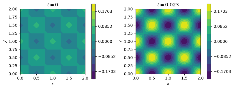
下面给出初始时刻和终止时刻的相场图.

The following plots show the phase field at the initial and final times.

limit = max(abs(u_initial.dat.data_ro).max(), abs(u_old.dat.data_ro).max())
levels = np.linspace(-limit, limit, 11)
fig, axes = plt.subplots(1, 2, figsize=(8, 3.3), constrained_layout=True)
for ax, uh, title in zip(axes, (u_initial, u_old), ('$t=0$', f'$t={num_steps*dt_value:.3f}$')):
    colors = tricontourf(uh, axes=ax, levels=levels)
    ax.set_aspect('equal')
    ax.set_xlabel('$x$')
    ax.set_ylabel('$y$')
    ax.set_title(title)
    _ = fig.colorbar(colors, ax=ax, shrink=0.82)

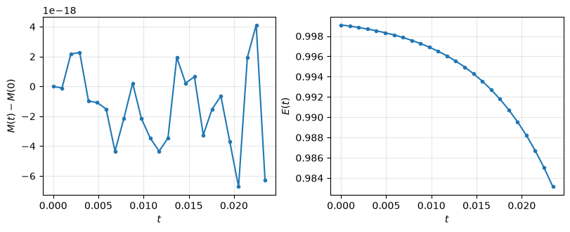
求解函数每一步记录质量和自由能. 下面检查离散质量守恒和自由能单调递减.

The solver function records mass and free energy at every step. We now check discrete mass conservation and monotone free-energy decay.

mass_error = np.max(np.abs(masses-masses[0]))
max_energy_increase = np.max(np.diff(energies))
print(f'maximum mass change = {mass_error:.3e}')
print(f'initial/final energy = {energies[0]:.8f} / {energies[-1]:.8f}')
print(f'maximum one-step energy increase = {max_energy_increase:.3e}')
assert mass_error < 1.0e-8
assert max_energy_increase < 1.0e-8

maximum mass change = 6.722e-18
initial/final energy = 0.99909979 / 0.98314547
maximum one-step energy increase = -1.183e-04

为清楚显示质量守恒误差, 左图画 \(M(t)-M(0)\). 数值结果表明质量变化保持在机器精度量级; 右图的自由能 \(E(t)\) 随时间单调降低, 与前述离散结构一致.

To expose the conservation error, the left panel plots \(M(t)-M(0)\). Its magnitude remains at the level of machine precision. The right panel shows that the free energy \(E(t)\) decreases monotonically in time, consistent with the discrete structure described above.

fig, axes = plt.subplots(1, 2, figsize=(8, 3.2), constrained_layout=True)
axes[0].plot(times, masses-masses[0], 'o-', markersize=3)
axes[0].set_xlabel('$t$')
axes[0].set_ylabel('$M(t)-M(0)$')
axes[0].ticklabel_format(axis='y', style='sci', scilimits=(0, 0))
axes[0].grid(alpha=0.3)

axes[1].plot(times, energies, 'o-', markersize=3)
axes[1].set_xlabel('$t$')
axes[1].set_ylabel('$E(t)$')
axes[1].grid(alpha=0.3)

4.4. 收敛阶测试 Convergence tests

为同时检查时间和空间离散, 在单位周期区域上取解

\[u(\boldsymbol x,t)=e^{-t}\cos(2\pi x)\cos(2\pi y),\qquad \mu=-\epsilon^2\Delta u+u^3-u.\]

方程源项可由解带入方程得到, 即 \(f=u_t-\Delta\mu\).

辅助函数 solve_ch_manufactured 在每个网格上构造 u_exact 和 source, 再把它们传给 solve_cahn_hilliard. 凸分裂时间格式预期为一阶; 对光滑解, 一次连续 Lagrange 元的 \(L^2\) 误差预期为二阶.

To test both temporal and spatial discretizations, use the manufactured solution

\[u(\boldsymbol x,t)=e^{-t}\cos(2\pi x)\cos(2\pi y),\qquad \mu=-\epsilon^2\Delta u+u^3-u\]

on the unit periodic domain. The source term is obtained by substituting the solution into the equation, i.e. \(f=u_t-\Delta\mu\). On each mesh, the helper solve_ch_manufactured constructs u_exact and source and passes them to solve_cahn_hilliard. The convex splitting is expected to be first order in time; for smooth solutions, continuous piecewise-linear elements are expected to be second order in the \(L^2\) norm.

def solve_ch_manufactured(N, num_steps, degree, T):
    mesh = PeriodicRectangleMesh(N, N, 1.0, 1.0)
    t = Constant(0.0)
    epsilon_value = 0.05
    x, y = SpatialCoordinate(mesh)
    u_exact = exp(-t)*cos(2*pi*x)*cos(2*pi*y)
    mu_exact = -epsilon_value**2*div(grad(u_exact)) + u_exact**3-u_exact
    source = -u_exact-div(grad(mu_exact))
    return solve_cahn_hilliard(
        mesh, num_steps, u_exact, degree=degree, T=T,
        epsilon_value=epsilon_value, source=source,
        u_exact=u_exact, time=t,
    )

def ch_error(result):
    error = result['u']-result['exact']
    return sqrt(assemble(error**2*dx(domain=result['mesh'], degree=5)))

def rates(errors, scales):
    result = [np.nan]
    for i in range(1, len(errors)):
        result.append(np.log(errors[i-1]/errors[i])/np.log(scales[i-1]/scales[i]))
    return np.asarray(result)

def print_convergence_table(title, headers, rows):
    rows = [[str(value) for value in row] for row in rows]
    widths = [
        max(len(header), *(len(row[j]) for row in rows))
        for j, header in enumerate(headers)
    ]
    print(title)
    print('  '.join(header.rjust(width) for header, width in zip(headers, widths)))
    for row in rows:
        print('  '.join(value.rjust(width) for value, width in zip(row, widths)))

def plot_convergence(ax, scales, errors, order, xlabel):
    scales = np.asarray(scales)
    errors = np.asarray(errors)
    reference = errors[-1]*(scales/scales[-1])**order
    ax.loglog(scales, errors, 'o-', label='error')
    ax.loglog(scales, reference, '--', label=fr'$O({xlabel}^{order})$')
    ax.set_xlabel(fr'${xlabel}$')
    ax.set_ylabel('$L^2$ error')
    ax.invert_xaxis()
    tick_indices = [0, len(scales)//2, len(scales)-1]
    ticks = scales[tick_indices]
    ax.set_xticks(ticks, [f'{value:.1e}' for value in ticks])
    ax.tick_params(axis='x', which='minor', labelbottom=False)
    ax.grid(which='both', alpha=0.3)
    ax.legend()

时间收敛测试固定网格并使用四次连续 Lagrange 元 (P4), 逐次减半时间步长, 以减小空间误差的影响. 空间收敛测试使用一次元 (P1), 并令 \(\tau\lesssim h^2/10\), 以减小时间误差的影响.

The temporal test fixes the mesh, uses quartic continuous Lagrange elements (P4), and successively halves the time step to reduce the influence of spatial error. The spatial test uses linear elements (P1) and sets \(\tau\lesssim h^2/10\) to reduce the influence of temporal error.

T_time = 0.0025
time_steps = np.asarray([4, 8, 16, 32])
time_sizes = T_time/time_steps
time_errors = np.asarray([
    ch_error(solve_ch_manufactured(16, steps, degree=4, T=T_time))
    for steps in time_steps
])
time_rates = rates(time_errors, time_sizes)

time_rows = [
    [steps, f'{dt_i:.3e}', f'{error:.3e}',
     '--' if np.isnan(rate) else f'{rate:.2f}']
    for steps, dt_i, error, rate
    in zip(time_steps, time_sizes, time_errors, time_rates)
]
print_convergence_table(
    'Temporal convergence', ['steps', 'dt', 'L2 error', 'rate'], time_rows
)

Temporal convergence
steps         dt   L2 error  rate
    4  6.250e-04  5.648e-05    --
    8  3.125e-04  2.915e-05  0.95
   16  1.563e-04  1.485e-05  0.97
   32  7.813e-05  7.540e-06  0.98

T_space = 0.001
space_N = np.asarray([16, 24, 32, 48])
space_h = 1.0/space_N
space_steps = np.ceil(10*T_space/space_h**2).astype(int)
space_errors = np.asarray([
    ch_error(solve_ch_manufactured(N_i, steps, degree=1, T=T_space))
    for N_i, steps in zip(space_N, space_steps)
])
space_rates = rates(space_errors, space_h)

space_rows = [
    [N_i, steps, f'{h_i:.3e}', f'{error:.3e}',
     '--' if np.isnan(rate) else f'{rate:.2f}']
    for N_i, steps, h_i, error, rate
    in zip(space_N, space_steps, space_h, space_errors, space_rates)
]
print_convergence_table(
    'Spatial convergence', ['N', 'steps', 'h', 'L2 error', 'rate'], space_rows
)

fig, axes = plt.subplots(1, 2, figsize=(8, 3.2), constrained_layout=True)
plot_convergence(axes[0], time_sizes, time_errors, 1, r'\tau')
plot_convergence(axes[1], space_h, space_errors, 2, 'h')

Spatial convergence
 N  steps          h   L2 error  rate
16      3  6.250e-02  1.536e-02    --
24      6  4.167e-02  6.965e-03  1.95
32     11  3.125e-02  3.958e-03  1.96
48     24  2.083e-02  1.773e-03  1.98

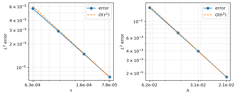
时间误差的观测阶约为 \(0.95\)–\(0.98\), 并随时间步长减小逐渐接近一阶; 空间误差的观测阶约为 \(1.95\)–\(1.98\), 与 P1 元的二阶 \(L^2\) 收敛率一致.

The observed temporal rates are about \(0.95\)–\(0.98\) and approach first order as the time step decreases. The observed spatial rates are about \(1.95\)–\(1.98\), consistent with second-order \(L^2\) convergence for P1 elements.

4.5. 随机初值算例 Example with a random initial condition

相分离计算通常从均匀混合态附近的小随机扰动开始. 先在有限元空间中生成区间 \([-0.05,0.05]\) 内的伪随机自由度值, 再减去数值平均值使初始总质量为零. 然后把该离散函数作为 initial 参数传给求解器. 下面代码中固定随机种子以使结果可复现.

Phase-separation simulations commonly start from a small random perturbation of a homogeneous mixture. We first generate pseudorandom degree-of-freedom values in \([-0.05,0.05]\) and subtract their numerical mean so that the initial total mass is zero. This discrete function is passed to the solver as initial; a fixed seed makes the result reproducible.

random_steps = 80
T_random = random_steps*2.0**(-10)
random_mesh = PeriodicRectangleMesh(24, 24, 2.0, 2.0)
V_random = FunctionSpace(random_mesh, 'CG', 1)
random_initial = Function(V_random)
rng = np.random.default_rng(2026)
random_initial.dat.data[:] = rng.uniform(
    -0.05, 0.05, size=random_initial.dat.data.shape
)
area = assemble(1*dx(domain=random_mesh))
random_initial.assign(random_initial-ch_mass(random_initial)/area)
random_result = solve_cahn_hilliard(
    random_mesh, random_steps, random_initial, degree=1, T=T_random
)
u_random_initial = random_result['initial']
u_random_final = random_result['u']
random_masses = random_result['masses']
random_energies = random_result['energies']

print(f'random initial mass = {random_masses[0]:.3e}')
print(f'random final mass   = {random_masses[-1]:.3e}')
print(f'random initial/final energy = {random_energies[0]:.8f} / {random_energies[-1]:.8f}')

random initial mass = -4.228e-18
random final mass   = 2.602e-17
random initial/final energy = 1.00144326 / 0.77299377

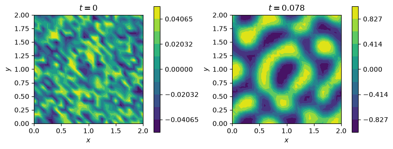
双井势的两个极小值位于 \(u=\pm1\). 下图的两幅图分别使用适合各自数据范围的色标: 初始随机扰动很小, 演化后相场逐渐形成分别趋向 \(+1\) 和 \(-1\) 的区域.

The two minima of the double-well potential are at \(u=\pm1\). The initial and final plots use color scales adapted to their respective data ranges: the initial random perturbation is small, while the evolved phase field develops regions tending toward \(+1\) and \(-1\).

fig, axes = plt.subplots(1, 2, figsize=(8, 3.3), constrained_layout=True)
for ax, uh, title in zip(
    axes, (u_random_initial, u_random_final),
    ('$t=0$', f'$t={T_random:.3f}$'),
):
    bound = abs(uh.dat.data_ro).max()
    colors = tricontourf(uh, axes=ax, levels=np.linspace(-bound, bound, 11))
    ax.set_aspect('equal')
    ax.set_xlabel('$x$')
    ax.set_ylabel('$y$')
    ax.set_title(title)
    _ = fig.colorbar(colors, ax=ax, shrink=0.82)

4.6. 二阶时间离散 (进阶) Second-order time discretization (advanced)

若希望时间方向达到二阶精度, 可以使用 BDF2 近似时间导数, 并用前两步的解外推凹项值:

For second-order accuracy in time, one may approximate the time derivative with BDF2 and extrapolate the concave term from the two previous solutions:

(4.8)\[\begin{equation} \frac{3u_h^{n+1}-4u_h^n+u_h^{n-1}}{2\tau},\qquad F'(u_h^{n+1})\approx (u_h^{n+1})^3-(2u_h^n-u_h^{n-1}). \end{equation}\]

实现时需要额外保存 \(u_h^{n-1}\), 并用上面的一阶格式启动. 二阶格式的能量稳定性依赖于具体分裂和稳定化项, 不能仅把时间差分替换为 BDF2 后直接沿用上面的能量断言; 二阶格式的稳定性与误差分析可参考 [SY10].

The implementation must store the additional state \(u_h^{n-1}\) and compute the first step with the first-order scheme above. Energy stability of a second-order method depends on the precise splitting and stabilization terms, so the energy assertion above cannot automatically be reused after merely replacing the time difference by BDF2; see [SY10] for stability and error analyses of second-order schemes.

References

[CH58] (1,2)

John W. Cahn and John E. Hilliard. Free energy of a nonuniform system. I. interfacial free energy. The Journal of Chemical Physics, 28(2):258–267, 1958. doi:10.1063/1.1744102.

[Eyr98] (1,2,3,4)

David J. Eyre. Unconditionally gradient stable time marching the Cahn–Hilliard equation. In Computational and Mathematical Models of Microstructural Evolution, volume 529 of Materials Research Society Symposium Proceedings, 39–46. Warrendale, PA, 1998. Materials Research Society. doi:10.1557/PROC-529-39.

[SY10] (1,2,3,4,5,6)

Jie Shen and Xiaofeng Yang. Numerical approximations of Allen–Cahn and Cahn–Hilliard equations. Discrete and Continuous Dynamical Systems, 28(4):1669–1691, 2010. doi:10.3934/dcds.2010.28.1669.