3. 抛物方程

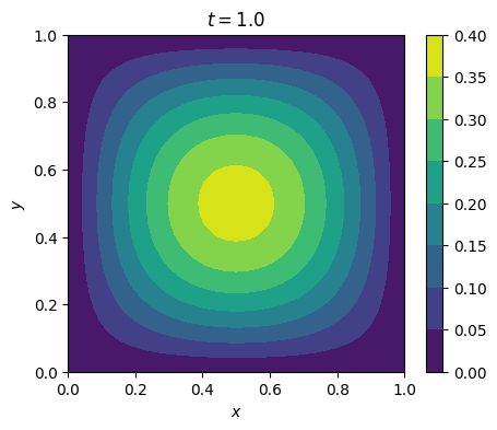
3.1. 固定区域

Consider the equation with Dirichlet boundary conditions

(3.1)\[\begin{equation} \left\{ \begin{aligned} &u_t - a\Delta u + (b \cdot \nabla) u- f = 0 \\ &u_0 = \phi(x) \\ &u_{\Gamma} = g(x) \end{aligned} \right. \end{equation}\]

on \(\Omega = [0, 1]^2\) with

(3.2)\[\begin{equation} \begin{aligned} &f = 0, \\ &g = 0, \\ &a = 1/(2\pi^2),\\ &b = (0, 0),\\ &\phi(x) = \sin(\pi x)\sin(\pi y). \\ \end{aligned} \end{equation}\]

The variational form is

(3.3)\[\begin{equation} F := (\frac{u^{n+1} - u^n}{\tau}, v) + (a\nabla u^{n+1}, \nabla v) + (b\cdot\nabla u^{n+1}, v) - (f^{n+1}, v) = 0 \end{equation}\]

3.1.1. Step to solve the problem

1. Define the domain/mesh

2. Create function space on the domain

3. Define the variational problem

   1. Define the variational form

   2. Define the boundary conditions

4. Define the variational solver

5. Solve the problem in a time loop

from firedrake import *
from firedrake.pyplot import tricontourf
import matplotlib.pyplot as plt


def plot_solution(u_h, time=None, vmin=None, vmax=None):
    fig, ax = plt.subplots(figsize=[5, 4])
    if vmin is None or vmax is None:
        levels = None
    else:
        levels = np.linspace(vmin, vmax, 11)
    cs = tricontourf(u_h, axes=ax, levels=levels)
    ax.set_aspect('equal')
    ax.set_xlabel('$x$')
    ax.set_ylabel('$y$')
    if time is not None:
        ax.set_title(f'$t={time}$')
    cbar = fig.colorbar(cs)


N = 32
M = 32
T = 1
dt = T/M

t = Constant(0)

a = Constant(1/(2*pi**2))
b = Constant([0, 0])
f = Constant(0)

mesh = UnitSquareMesh(N, N)
x, y = SpatialCoordinate(mesh)
u_0 = sin(pi*x)*sin(pi*y)

V = FunctionSpace(mesh, 'CG', 1)
u_trial, u_test = TrialFunction(V), TestFunction(V)
u_n = Function(V, name='u_n')
u_h = Function(V, name='u_h')

bc = DirichletBC(V, 0, 'on_boundary')

A = (
    1/dt*(u_trial - u_n)*u_test*dx
    + inner(grad(u_trial), b*u_test)*dx
    + inner(a*grad(u_trial), grad(u_test))*dx
    - f*u_test*dx
)

problem = LinearVariationalProblem(lhs(A), rhs(A), u_h, bcs=bc)
solver = LinearVariationalSolver(problem)

u_h.project(u_0)
# u_h.interpolate(u_0)
u_n.assign(u_h)

plot_solution(u_h, time=0)

# output = VTKFile('result.pvd', adaptive=True)
# output.write(u_h, time=0)

for i in range(M):
    t.assign((i+1)*dt)
    solver.solve()
    u_n.assign(u_h)
    # output.write(u_h, time=float(t))

plot_solution(u_h, time=float(t))

3.1.2. Run the code

Save the code to file heat.py, and run it as follows.

python heat.py
mpiexec -n 4 python heat.py

Add command line options

1. petsc options

2. custom options

3.1.3. View results in paraview

Download paraview from https://www.paraview.org/download/.

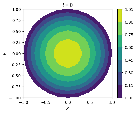
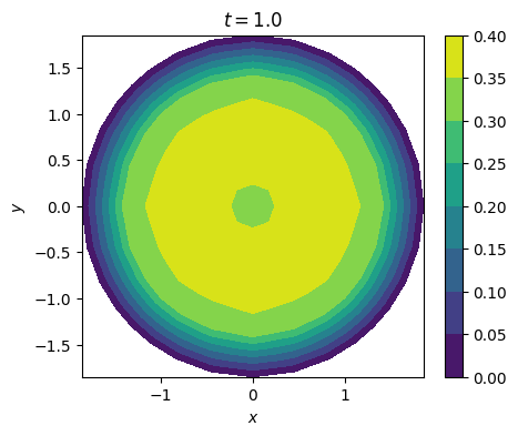
3.2. 移动边界问题

from firedrake import *
from firedrake.pyplot import tricontourf
import matplotlib.pyplot as plt


def plot_solution(u_h, time=None, vmin=None, vmax=None):
    fig, ax = plt.subplots(figsize=[5, 4])
    if vmin is None or vmax is None:
        levels = None
    else:
        levels = np.linspace(vmin, vmax, 11)
    cs = tricontourf(u_h, axes=ax, levels=levels)
    ax.set_aspect('equal')
    ax.set_xlabel('$x$')
    ax.set_ylabel('$y$')
    if time is not None:
        ax.set_title(f'$t={time}$')
    cbar = fig.colorbar(cs)


T = 1
M = 32
dt = 1/M

a = Constant(1)
b = as_vector([0, 0]) # vector([0, 0, 0])

t = Constant(0)

mesh = UnitDiskMesh(2)
# mesh = Mesh(gmshfile)
x, y = SpatialCoordinate(mesh)
f = x**2 + y**2
u_0 = 1 - x**2 - y**2
v = as_vector([x, y])*exp(-t)

V_coords = VectorFunctionSpace(mesh, 'CG', 1)
w_vel = Function(V_coords)

V = FunctionSpace(mesh, 'CG', 1)
u_trial, u_test = TrialFunction(V), TestFunction(V)
u_n = Function(V, name='u_n')
u_h = Function(V, name='u_h')

bc = DirichletBC(V, 0, 'on_boundary')

A = (
    1/dt*(u_trial - u_n)*u_test*dx
    + inner(grad(u_trial), u_test*(b - w_vel))*dx
    + inner(a*grad(u_trial), grad(u_test))*dx
    - f*u_test*dx
)

problem = LinearVariationalProblem(lhs(A), rhs(A), u_h, bcs=bc)
solver = LinearVariationalSolver(problem)

w_trial, w_test = TrialFunction(V_coords), TestFunction(V_coords)
bc_move_mesh = DirichletBC(V_coords, v, 'on_boundary')
B = inner(grad(w_trial), grad(w_test))*dx - Constant(0)*w_test[0]*dx

mm_problem = LinearVariationalProblem(lhs(B), rhs(B), w_vel, bcs=bc_move_mesh)
mm_solver = LinearVariationalSolver(mm_problem)

u_h.project(u_0)
# u_h.interpolate(u_0)
u_n.assign(u_h)

# output = VTKFile('result.pvd', adaptive=True)
# output.write(u_h, time=0)

plot_solution(u_h, time=0)

for i in range(M):
    t.assign((i+1)*dt)

    mm_solver.solve()
    mesh.coordinates.assign(mesh.coordinates + dt*w_vel)

    solver.solve()
    u_n.assign(u_h)
    # output.write(u_h, time=(i+1)*dt)

plot_solution(u_h, time=M*dt)