5. Navier–Stokes 方程 The Navier–Stokes Equations

本章内容

本章以二维顶盖驱动方腔流为例求解不可压 Navier–Stokes 方程. 先给出完整问题及其弱形式, 再介绍速度–压力空间、非线性残量、边界条件、压力零空间和时间求解.

Overview

This chapter solves the two-dimensional lid-driven cavity problem for the incompressible Navier–Stokes equations. We first state the complete problem and its weak form, and then introduce the velocity–pressure space, nonlinear residual, boundary conditions, pressure nullspace, and time stepping.

5.1. 方程与弱形式 Equations and weak form

设 \(\Omega\subset\mathbb R^2\) 为有界区域. 不可压 Navier–Stokes 方程为

Let \(\Omega\subset\mathbb R^2\) be a bounded domain. The incompressible Navier–Stokes equations are

(5.1)\[\begin{equation} \begin{aligned} \partial_t\boldsymbol u-\nu\Delta\boldsymbol u +(\boldsymbol u\cdot\nabla)\boldsymbol u+\nabla p&=\boldsymbol f,\\ \nabla\cdot\boldsymbol u&=0. \end{aligned} \end{equation}\]

其中 \(\boldsymbol u\) 是速度, \(p\) 是压力, \(\nu>0\) 是运动黏度, \(\boldsymbol f\) 是体力.

Here \(\boldsymbol u\) is velocity, \(p\) is pressure, \(\nu>0\) is the kinematic viscosity, and \(\boldsymbol f\) is a body force.

设速度满足 Dirichlet 边界条件 \(\boldsymbol u=\boldsymbol g\), 并定义

Suppose that the velocity satisfies the Dirichlet condition \(\boldsymbol u=\boldsymbol g\), and define

(5.2)\[\begin{equation} \boldsymbol V_{\boldsymbol g}=\{\boldsymbol v\in[H^1(\Omega)]^2:\boldsymbol v|_{\partial\Omega}=\boldsymbol g\},\quad \boldsymbol V_0=[H_0^1(\Omega)]^2,\quad Q=L^2(\Omega)/\mathbb R. \end{equation}\]

对动量方程分部积分, 并用检验函数 \(\boldsymbol v\in\boldsymbol V_0\) 消去边界项. 连续弱形式为: 求 \((\boldsymbol u(t),p(t))\in\boldsymbol V_{\boldsymbol g}\times Q\), 使对任意 \((\boldsymbol v,q)\in\boldsymbol V_0\times Q\),

Integrating the momentum equation by parts and using \(\boldsymbol v\in\boldsymbol V_0\) removes the boundary term. The continuous weak problem is: find \((\boldsymbol u(t),p(t))\in\boldsymbol V_{\boldsymbol g}\times Q\) such that, for every \((\boldsymbol v,q)\in\boldsymbol V_0\times Q\),

(5.3)\[\begin{equation} (\partial_t\boldsymbol u,\boldsymbol v)+\nu(\nabla\boldsymbol u,\nabla\boldsymbol v) +c(\boldsymbol u;\boldsymbol u,\boldsymbol v)-(p,\nabla\cdot\boldsymbol v) +(q,\nabla\cdot\boldsymbol u)=(\boldsymbol f,\boldsymbol v), \end{equation}\]

(5.4)\[\begin{equation} c(\boldsymbol w;\boldsymbol u,\boldsymbol v) =\frac12\big((\boldsymbol w\cdot\nabla\boldsymbol u,\boldsymbol v) -(\boldsymbol w\cdot\nabla\boldsymbol v,\boldsymbol u)\big). \end{equation}\]

取满足离散 inf–sup 条件的有限元空间 \(\boldsymbol V_{\boldsymbol g,h}\subset\boldsymbol V_{\boldsymbol g}\), \(\boldsymbol V_{0,h}\subset\boldsymbol V_0\) 和 \(Q_h\subset Q\). 对时间导数使用后向 Euler 格式. 设 \(t_n=n\tau\), 每一步求 \((\boldsymbol u_h^{n+1},p_h^{n+1})\in\boldsymbol V_{\boldsymbol g,h}\times Q_h\), 使对任意 \((\boldsymbol v_h,q_h)\in\boldsymbol V_{0,h}\times Q_h\),

Let \(\boldsymbol V_{\boldsymbol g,h}\subset\boldsymbol V_{\boldsymbol g}\), \(\boldsymbol V_{0,h}\subset\boldsymbol V_0\), and \(Q_h\subset Q\) be finite element spaces satisfying the discrete inf–sup condition. We use backward Euler for the time derivative. With \(t_n=n\tau\), each step seeks \((\boldsymbol u_h^{n+1},p_h^{n+1})\in\boldsymbol V_{\boldsymbol g,h}\times Q_h\) such that, for every \((\boldsymbol v_h,q_h)\in\boldsymbol V_{0,h}\times Q_h\),

(5.5)\[\begin{equation} \begin{aligned} \left(\frac{\boldsymbol u_h^{n+1}-\boldsymbol u_h^n}{\tau},\boldsymbol v_h\right) +\nu(\nabla\boldsymbol u_h^{n+1},\nabla\boldsymbol v_h) +c(\boldsymbol u_h^{n+1};\boldsymbol u_h^{n+1},\boldsymbol v_h) -(p_h^{n+1},\nabla\cdot\boldsymbol v_h) +(q_h,\nabla\cdot\boldsymbol u_h^{n+1}) &=(\boldsymbol f,\boldsymbol v_h). \end{aligned} \end{equation}\]

反对称对流形式满足 \(c(\boldsymbol w;\boldsymbol u,\boldsymbol u)=0\), 不会对离散动能产生非物理贡献. 对流速度取新时间层的 \(\boldsymbol u_h^{n+1}\), 因而每个时间步都是非线性问题.

The skew-symmetric convection form satisfies \(c(\boldsymbol w;\boldsymbol u,\boldsymbol u)=0\) and therefore makes no spurious contribution to discrete kinetic energy. The convecting velocity is evaluated at the new time level, so every time step is nonlinear.

下面以顶盖驱动方腔流为例进行求解. 取 \(\Omega=(0,1)^2\), \(\nu=1\), \(\boldsymbol f=0\) 和零初值. 记上边界为 \(\Gamma_{\mathrm{lid}}\), 其余三条边界为 \(\Gamma_{\mathrm{wall}}\), 则

We now solve a lid-driven cavity problem. Take \(\Omega=(0,1)^2\), \(\nu=1\), \(\boldsymbol f=0\), and a zero initial condition. Denote the top boundary by \(\Gamma_{\mathrm{lid}}\) and the other three sides by \(\Gamma_{\mathrm{wall}}\). Then

(5.6)\[\begin{equation} \boldsymbol u=(1,0)\quad\text{on }\Gamma_{\mathrm{lid}},\qquad \boldsymbol u=\boldsymbol 0\quad\text{on }\Gamma_{\mathrm{wall}},\qquad \boldsymbol u(\cdot,0)=\boldsymbol 0. \end{equation}\]

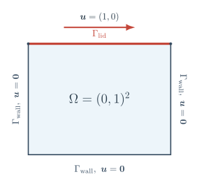
Fig. 5.1 顶盖驱动方腔流的求解区域与边界条件. Computational domain and boundary conditions for lid-driven cavity flow.

上方两个角点处的边界数据不连续; 这是经典方腔流算例的一部分. 数值实现中按边界标记直接施加这些数据; 若需要满足标准 \(H^1\) 弱形式对边界数据的正则性要求, 可在两个角点附近对顶盖速度作平滑化.

The boundary data are discontinuous at the two upper corners; this is part of the classical lid-driven cavity benchmark. The data are imposed directly by boundary markers in the numerical implementation. To meet the regularity assumptions of the standard \(H^1\) weak formulation, one may instead smooth the lid velocity near the two corners.

5.2. 网格、空间与变分问题 Mesh, spaces, and the variational problem

5.2.1. 网格与参数 Mesh and parameters

使用 UnitSquareMesh(16, 16) 生成的均匀三角形网格, 将终止时间 \(T=1/8\) 等分为 16 个时间步. dt 和 nu 定义为 Constant, 使它们可直接参与 UFL 形式的组装.

We use the uniform triangular mesh generated by UnitSquareMesh(16, 16) and divide the final time \(T=1/8\) into 16 steps. Defining dt and nu as Constant objects allows them to appear directly in the assembled UFL form.

from firedrake import *
from firedrake.pyplot import streamplot, tricontour
import matplotlib.pyplot as plt
import numpy as np

nu = Constant(1.0)
T = 1.0/8.0
num_steps = 16
dt_value = T/num_steps
dt = Constant(dt_value)

mesh = UnitSquareMesh(16, 16)
body_force = Constant((0.0, 0.0))

5.2.2. Taylor–Hood 速度–压力空间 The Taylor–Hood velocity–pressure space

速度和压力空间不能任意组合, 而应满足离散 inf–sup 条件. 本例先使用 Taylor–Hood 元: 速度采用连续分片二次空间 \([P_2]^2\), 压力采用连续分片一次空间 \(P_1\). V_u * V_p 构造速度–压力乘积空间. split(state) 返回用于组装 UFL 形式的符号分量, state_old.subfunctions 则返回可以赋值、计算和输出的 Function 分量.

The velocity and pressure spaces cannot be chosen independently; they should satisfy a discrete inf–sup condition. We first use Taylor–Hood elements: continuous piecewise quadratics \([P_2]^2\) for velocity and continuous piecewise linears \(P_1\) for pressure. V_u * V_p constructs the velocity–pressure product space. split(state) returns symbolic components for assembling UFL forms, whereas state_old.subfunctions returns Function components that can be assigned, evaluated, and written.

进阶: 使用 MINI 元 Advanced: using the MINI element

MINI 元是另一个满足 inf–sup 条件的速度–压力对. 压力仍使用 \(P_1\), 速度则使用 \([P_1^b]^2\), 其中 \(P_1^b=P_1\oplus B_3\). \(B_3\) 由三角形单元内的三次泡函数张成; 泡函数在单元边界上为零, 为每个速度分量增加一个单元内部自由度.

将下面主程序中定义 V_u 和 V_p 的两行替换为:

The MINI element is another inf–sup stable velocity–pressure pair. Pressure still uses \(P_1\), while velocity uses \([P_1^b]^2\), where \(P_1^b=P_1\oplus B_3\). The space \(B_3\) is spanned by the cubic bubble on each triangle. This bubble vanishes on the element boundary and adds one cell-interior degree of freedom to each velocity component.

Replace the two lines defining V_u and V_p in the main program by:

cell = mesh.ufl_cell()
P1 = FiniteElement("Lagrange", cell, 1)
bubble = FiniteElement("Bubble", cell, 3)
P1b = P1 + bubble
V_u = VectorFunctionSpace(mesh, P1b)
V_p = FunctionSpace(mesh, P1)

后续混合空间、残量和求解器代码均无需改动.

The remaining mixed-space, residual, and solver code is unchanged.

V_u = VectorFunctionSpace(mesh, 'CG', 2)
V_p = FunctionSpace(mesh, 'CG', 1)
Z = V_u * V_p

state = Function(Z, name='state')
u, p = split(state)
v, q = TestFunctions(Z)

state_old = Function(Z, name='state_old')
u_old, p_old = state_old.subfunctions
u_old.rename('velocity')
p_old.rename('pressure')
state_old.assign(0)

Coefficient(WithGeometry(MixedFunctionSpace(IndexedProxyFunctionSpace(<firedrake.mesh.MeshTopology object at 0x7f7afce4e4b0>, VectorElement(FiniteElement('Lagrange', triangle, 2), dim=2), name=None, index=0, component=None), IndexedProxyFunctionSpace(<firedrake.mesh.MeshTopology object at 0x7f7afce4e4b0>, FiniteElement('Lagrange', triangle, 1), name=None, index=1, component=None), name='None_None'), MeshSequence((Mesh(VectorElement(FiniteElement('Lagrange', triangle, 1), dim=2), 1), Mesh(VectorElement(FiniteElement('Lagrange', triangle, 1), dim=2), 1)))), 8)

5.2.3. 非线性残量 Nonlinear residual

state 是当前时间层的未知量, state_old 保存上一时间层的数值解. 代码中的 residual 依次对应时间导数、黏性项、反对称对流项的两部分、压力项、不可压约束和体力. 在 UFL 中, dot(grad(u), u) 表示 \((\boldsymbol u\cdot\nabla)\boldsymbol u\), 而 dot(grad(v), u) 表示 \((\boldsymbol u\cdot\nabla)\boldsymbol v\).

state is the unknown at the current time level, whereas state_old stores the numerical solution from the preceding level. The terms in residual represent, in order, the time derivative, viscosity, the two halves of the skew-symmetric convection form, pressure, incompressibility, and body force. In UFL, dot(grad(u), u) represents \((\boldsymbol u\cdot\nabla)\boldsymbol u\), while dot(grad(v), u) represents \((\boldsymbol u\cdot\nabla)\boldsymbol v\).

residual = (
    inner((u-u_old)/dt, v)*dx
    + nu*inner(grad(u), grad(v))*dx
    + 0.5*inner(dot(grad(u), u), v)*dx
    - 0.5*inner(dot(grad(v), u), u)*dx
    - p*div(v)*dx
    + q*div(u)*dx
    - inner(body_force, v)*dx
)

5.2.4. 边界条件与压力零空间 Boundary conditions and the pressure nullspace

UnitSquareMesh 的边界编号依次为左、右、下、上边界 \(1,2,3,4\). 边界条件只施加在混合空间的速度分量 Z.sub(0) 上. 压力没有边界条件, 且方程只含 \(\nabla p\), 因而压力只确定到一个加法常数.

MixedVectorSpaceBasis 表明速度分量没有零空间, 压力分量的常数函数构成零空间. 这让线性求解器正确处理每次 Newton 迭代中的奇异 Jacobian; 它并不是额外的压力边界条件.

The boundary markers of UnitSquareMesh are \(1,2,3,4\) for the left, right, bottom, and top sides. Boundary conditions are imposed only on the velocity component Z.sub(0) of the mixed space. Pressure has no boundary condition, and because only \(\nabla p\) occurs in the equations, it is determined only up to an additive constant.

MixedVectorSpaceBasis specifies that the velocity block has no nullspace while constant functions span the pressure nullspace. This allows the linear solver to handle the singular Jacobian in each Newton iteration correctly; it is not an additional pressure boundary condition.

bc_walls = DirichletBC(Z.sub(0), Constant((0.0, 0.0)), (1, 2, 3))
bc_lid = DirichletBC(Z.sub(0), Constant((1.0, 0.0)), 4)
bcs = [bc_walls, bc_lid]

nullspace = MixedVectorSpaceBasis(
    Z, [Z.sub(0), VectorSpaceBasis(constant=True, comm=mesh.comm)]
)
problem = NonlinearVariationalProblem(residual, state, bcs=bcs)

5.3. 求解器配置 Solver configuration

NonlinearVariationalSolver 在每个时间步用 SNES 求解非线性问题, Newton 迭代中的 Jacobian 线性系统则由 KSP 和 PC 处理. 小规模问题适合直接法, 实现简单且稳健; 网格加密后, 通常应改用针对速度–压力块结构设计的迭代法.

At each time step, NonlinearVariationalSolver uses SNES for the nonlinear problem, while KSP and PC handle the Jacobian system arising in each Newton iteration. A direct method is simple and robust for small problems; on refined meshes, an iterative method designed around the velocity–pressure block structure is usually preferable.

5.3.1. 直接法 Direct method

本例默认采用 preonly + LU 直接法. 由于 nullspace 不参与 LU 分解, 这里显式选用 MUMPS, 并以 ICNTL(24)=1 开启零主元检测、以 CNTL(3)=10^{-12} 设置相对阈值系数. MUMPS 参数负责处理奇异矩阵的分解, nullspace 则使 KSP 在应用预条件子后投影掉压力的常数分量.

This example uses a preonly + LU direct solve by default. Because nullspace does not participate in the LU factorization, we explicitly select MUMPS, enable null-pivot detection with ICNTL(24)=1, and set the relative threshold coefficient to CNTL(3)=10^{-12}. The MUMPS options handle the factorization of the singular matrix, while nullspace makes KSP project out the constant pressure component after applying the preconditioner.

direct_parameters = {
    'snes_error_if_not_converged': True,
    'ksp_type': 'preonly',
    'pc_type': 'lu',
    'pc_factor_mat_solver_type': 'mumps',
    'mat_mumps_icntl_24': 1,
    'mat_mumps_cntl_3': 1e-12,
}
solver = NonlinearVariationalSolver(
    problem, options_prefix='ns', nullspace=nullspace,
    solver_parameters=direct_parameters,
)

5.3.2. 迭代法 Iterative method

网格加密后, 直接分解的计算量和内存开销增长较快. 对速度–压力鞍点系统, 更合适的迭代方案是用 fieldsplit 构造 Schur 补块预条件子. 下面使用外层 FGMRES: 速度块通过 AssembledPC 组装后用 Hypre AMG 近似求逆, 压力 Schur 补则用 Firedrake 的压力对流–扩散预条件子 PCDPC 近似. 由于压力块本身还包含非定常的内层 GMRES, 外层采用允许预条件子变化的 FGMRES.

PCDPC 还需要从 appctx 取得当前状态、Reynolds 数和速度在混合空间中的编号. 本例 ν = 1, 因而 Re = 1/ν = 1. 在当前 16 × 16 网格上, 实测中每次 Newton 线性化约需 8 次外层 FGMRES 迭代; 这一数值会随网格、参数和容差变化. 以下配置参考 Firedrake 的 Navier–Stokes 示例. 这里将迭代求解器命名为 iterative_solver; 若要在后面的时间循环中采用它, 将循环内的 solver.solve() 改为 iterative_solver.solve() 即可.

For refined meshes, the cost and memory consumption of direct factorization grow rapidly. A more appropriate iterative method for the velocity–pressure saddle-point system uses fieldsplit to construct a Schur-complement block preconditioner. The configuration below uses outer FGMRES: the velocity block is assembled through AssembledPC and approximately inverted by Hypre AMG, while Firedrake’s pressure convection–diffusion preconditioner PCDPC approximates the pressure Schur complement. Since the pressure block contains a nonstationary inner GMRES solve, flexible GMRES is used on the outside.

PCDPC also obtains the current state, Reynolds number, and the index of the velocity field from appctx. Here ν = 1, so Re = 1/ν = 1. On the present 16 × 16 mesh, our tests required about eight outer FGMRES iterations for each Newton linearization; this count depends on the mesh, parameters, and tolerances. The configuration is based on the Firedrake Navier–Stokes demo. The iterative solver is named iterative_solver; to use it in the time loop of the next section, replace solver.solve() by iterative_solver.solve().

iterative_parameters = {
    'snes_error_if_not_converged': True,
    'mat_type': 'matfree',
    'ksp_type': 'fgmres',
    'ksp_rtol': 1e-8,
    'ksp_max_it': 100,
    'ksp_error_if_not_converged': True,
    'pc_type': 'fieldsplit',
    'pc_fieldsplit_type': 'schur',
    'pc_fieldsplit_schur_fact_type': 'lower',
    'fieldsplit_0_ksp_type': 'preonly',
    'fieldsplit_0_pc_type': 'python',
    'fieldsplit_0_pc_python_type': 'firedrake.AssembledPC',
    'fieldsplit_0_assembled_pc_type': 'hypre',
    'fieldsplit_1_ksp_type': 'gmres',
    'fieldsplit_1_ksp_rtol': 1e-3,
    'fieldsplit_1_pc_type': 'python',
    'fieldsplit_1_pc_python_type': 'firedrake.PCDPC',
    'fieldsplit_1_pcd_Mp_ksp_type': 'preonly',
    'fieldsplit_1_pcd_Mp_pc_type': 'jacobi',
    'fieldsplit_1_pcd_Kp_ksp_type': 'preonly',
    'fieldsplit_1_pcd_Kp_pc_type': 'hypre',
    'fieldsplit_1_pcd_Fp_mat_type': 'matfree',
}

iterative_solver = NonlinearVariationalSolver(
    problem, options_prefix='ns', nullspace=nullspace,
    solver_parameters=iterative_parameters,
    appctx={'state': state, 'Re': Constant(1.0),
            'velocity_space': 0},
)

5.4. 求解与结果检查 Solution and result checks

时间循环、时变系数、PVD 输出和 ParaView 操作的通用写法已在热传导方程一章中介绍, 参见 相关小节. 这里仅保留 NS 方程特有的步骤: 用旧的速度–压力状态初始化非线性迭代, 求出新状态后更新 state_old. 第一个时间步求解完成后, 使用 ASCII_INFO_DETAIL 格式输出 SNES、KSP 和 PC 的详细配置; 随后直接查询 Jacobian 矩阵, 确认压力零空间已挂载.

最后输出速度散度的 \(L^2\) 范数和动能. Taylor–Hood 元只在压力空间意义下满足不可压约束, 因此 div(u_old) 一般不会逐点为零; 该数值主要用于网格和格式之间的比较, 不应断言为机器零.

The common treatment of time loops, time-dependent coefficients, PVD output, and ParaView was introduced in the heat-equation chapter; see the corresponding section. Here we retain only the steps specific to the Navier–Stokes problem: initialize the nonlinear iteration with the old velocity–pressure state, solve for the new state, and update state_old. After the first time step, we use the ASCII_INFO_DETAIL format to report the detailed SNES, KSP, and PC configuration; we then query the Jacobian matrix directly to verify that the pressure nullspace is attached.

We finally report the \(L^2\) norm of the velocity divergence and the kinetic energy. Taylor–Hood elements enforce incompressibility only in the pressure-space weak sense, so div(u_old) is generally not pointwise zero; the value is useful for comparisons between meshes and schemes but should not be asserted to be machine zero.

for step in range(num_steps):
    state.assign(state_old)
    solver.solve()
    if step == 0:
        PETSc.Sys.Print('Solver configuration after the first time step:')
        viewer = PETSc.Viewer.STDOUT(mesh.comm)
        viewer.pushFormat(PETSc.Viewer.Format.ASCII_INFO_DETAIL)
        solver.snes.view(viewer)
        viewer.popFormat()
        jacobian = solver.snes.getJacobian()[0]
        nullspace_attached = jacobian.getNullSpace() is not None
        PETSc.Sys.Print(f'Jacobian nullspace attached = {nullspace_attached}')
    state_old.assign(state)

Show code cell output

Hide code cell output

Solver configuration after the first time step:
SNES Object: (ns_) 1 MPI process
  type: newtonls
  maximum iterations=50, maximum function evaluations=10000
  tolerances: relative=1e-08, absolute=1e-50, solution=1e-08
  total number of linear solver iterations=2
  total number of function evaluations=3
  norm schedule ALWAYS
  SNESLineSearch Object: (ns_) 1 MPI process
    type: basic
    maxlambda=1.000000e+00, minlambda=1.000000e-12
    tolerances: relative=1.000000e-08, absolute=1.000000e-15, lambda=1.000000e-08
    maximum iterations=40
  KSP Object: (ns_) 1 MPI process
    type: preonly
    maximum iterations=10000, initial guess is zero
    tolerances: relative=1e-05, absolute=1e-50, divergence=10000.
    left preconditioning
    not checking for convergence
  PC Object: (ns_) 1 MPI process
    type: lu
      out-of-place factorization
      tolerance for zero pivot 2.22045e-14
      matrix ordering: external
      factor fill ratio given 0., needed 0.        Factored matrix:
          Mat Object: (ns_) 1 MPI process
            type: mumps
            rows=2467, cols=2467
            package used to perform factorization: mumps
            total: nonzeros=308447, allocated nonzeros=308447
              MUMPS run parameters:
                SYM (matrix type):                   0
                PAR (host participation):            1
                ICNTL(1) (output for error):         6
                ICNTL(2) (output of diagnostic msg): 0
                ICNTL(3) (output for global info):   0
                ICNTL(4) (level of printing):        0
                ICNTL(5) (input mat struct):         0
                ICNTL(6) (matrix prescaling):        7
                ICNTL(7) (sequential matrix ordering):7
                ICNTL(8) (scaling strategy):         77
                ICNTL(10) (max num of refinements):  0
                ICNTL(11) (error analysis):          0
                ICNTL(12) (efficiency control):                         1
                ICNTL(13) (sequential factorization of the root node):  1
                ICNTL(14) (percentage of estimated workspace increase): 20
                ICNTL(15) (compression of the input matrix):            0
                ICNTL(18) (input mat struct):                           0
                ICNTL(19) (Schur complement info):                      0
                ICNTL(20) (RHS sparse pattern):                         0
                ICNTL(21) (solution struct):                            0
                ICNTL(22) (in-core/out-of-core facility):               0
                ICNTL(23) (max size of memory can be allocated locally):0
                ICNTL(24) (detection of null pivot rows):               1
                ICNTL(25) (computation of a null space basis):          0
                ICNTL(26) (Schur options for RHS or solution):          0
                ICNTL(27) (blocking size for multiple RHS):             -32
                ICNTL(28) (use parallel or sequential ordering):        1
                ICNTL(29) (parallel ordering):                          0
                ICNTL(30) (user-specified set of entries in inv(A)):    0
                ICNTL(31) (factors is discarded in the solve phase):    0
                ICNTL(33) (compute determinant):                        0
                ICNTL(35) (activate BLR based factorization):           0
                ICNTL(36) (choice of BLR factorization variant):        0
                ICNTL(37) (compression of the contribution blocks):     0
                ICNTL(38) (estimated compression rate of LU factors):   600
                ICNTL(48) (multithreading with tree parallelism):       0
                ICNTL(49) (compact workarray at the end of factorization phase):0
                ICNTL(56) (postponing and rank-revealing factorization):0
                ICNTL(58) (options for symbolic factorization):         2
                CNTL(1) (relative pivoting threshold):      0.01
                CNTL(2) (stopping criterion of refinement): 1.49012e-08
                CNTL(3) (absolute pivoting threshold):      1e-12
                CNTL(4) (value of static pivoting):         -1.
                CNTL(5) (fixation for null pivots):         0.
                CNTL(7) (dropping parameter for BLR):       0.
                RINFO(1) (local estimated flops for the elimination after analysis):
                  [0] 2.31077e+07
                RINFO(2) (local estimated flops for the assembly after factorization):
                  [0] 308751.
                RINFO(3) (local estimated flops for the elimination after factorization):
                  [0] 2.31077e+07
                INFO(15) (estimated size of (in MB) MUMPS internal data for running numerical factorization):
                  [0] 4
                INFO(16) (size of (in MB) MUMPS internal data used during numerical factorization):
                  [0] 4
                INFO(23) (num of pivots eliminated on this processor after factorization):
                  [0] 2467
                RINFOG(1) (global estimated flops for the elimination after analysis): 2.31077e+07
                RINFOG(2) (global estimated flops for the assembly after factorization): 308751.
                RINFOG(3) (global estimated flops for the elimination after factorization): 2.31077e+07
                (RINFOG(12) RINFOG(13))*2^INFOG(34) (determinant): (0.,0.)*(2^0)                INFOG(3) (estimated real workspace for factors on all processors after analysis): 308447
                INFOG(4) (estimated integer workspace for factors on all processors after analysis): 19308
                INFOG(5) (estimated maximum front size in the complete tree): 159
                INFOG(6) (number of nodes in the complete tree): 133
                INFOG(7) (ordering option effectively used after analysis): 2
                INFOG(8) (structural symmetry in percent of the permuted matrix after analysis): 100
                INFOG(9) (total real/complex workspace to store the matrix factors after factorization): 308447
                INFOG(10) (total integer space store the matrix factors after factorization): 19308
                INFOG(11) (order of largest frontal matrix after factorization): 159
                INFOG(12) (number of off-diagonal pivots): 2
                INFOG(13) (number of delayed pivots after factorization): 0
                INFOG(14) (number of memory compress after factorization): 0
                INFOG(15) (number of steps of iterative refinement after solution): 0
                INFOG(16) (estimated size (in MB) of all MUMPS internal data for factorization after analysis: value on the most memory consuming processor): 4
                INFOG(17) (estimated size of all MUMPS internal data for factorization after analysis: sum over all processors): 4
                INFOG(18) (size of all MUMPS internal data allocated during factorization: value on the most memory consuming processor): 4
                INFOG(19) (size of all MUMPS internal data allocated during factorization: sum over all processors): 4
                INFOG(20) (estimated number of entries in the factors): 308447
                INFOG(21) (size in MB of memory effectively used during factorization - value on the most memory consuming processor): 4
                INFOG(22) (size in MB of memory effectively used during factorization - sum over all processors): 4
                INFOG(23) (after analysis: value of ICNTL(6) effectively used): 0
                INFOG(24) (after analysis: value of ICNTL(12) effectively used): 1
                INFOG(25) (after factorization: number of pivots modified by static pivoting): 0
                INFOG(28) (after factorization: number of null pivots encountered): 1
                INFOG(29) (after factorization: effective number of entries in the factors (sum over all processors)): 308447
                INFOG(30, 31) (after solution: size in Mbytes of memory used during solution phase): 3, 3
                INFOG(32) (after analysis: type of analysis done): 1
                INFOG(33) (value used for ICNTL(8)): 7
                INFOG(34) (exponent of the determinant if determinant is requested): 0
                INFOG(35) (after factorization: number of entries taking into account BLR factor compression - sum over all processors): 308447
                INFOG(36) (after analysis: estimated size of all MUMPS internal data for running BLR in-core - value on the most memory consuming processor): 0
                INFOG(37) (after analysis: estimated size of all MUMPS internal data for running BLR in-core - sum over all processors): 0
                INFOG(38) (after analysis: estimated size of all MUMPS internal data for running BLR out-of-core - value on the most memory consuming processor): 0
                INFOG(39) (after analysis: estimated size of all MUMPS internal data for running BLR out-of-core - sum over all processors): 0
    linear system matrix, which is also used to construct the preconditioner:
    Mat Object: (ns_) 1 MPI process
      type: seqaij
      rows=2467, cols=2467
      total: nonzeros=68521, allocated nonzeros=68521
      total number of mallocs used during MatSetValues calls=0
        has attached null space
        using I-node routines: found 1376 nodes, limit used is 5
Jacobian nullspace attached = True

divergence_L2 = sqrt(assemble(div(u_old)**2*dx))
kinetic_energy = assemble(0.5*inner(u_old, u_old)*dx)
print(f'final time = {T:.3f}')
print(f'L2 norm of divergence = {divergence_L2:.3e}')
print(f'kinetic energy = {kinetic_energy:.3e}')
assert np.isfinite(divergence_L2) and kinetic_energy > 0

final time = 0.125
L2 norm of divergence = 3.709e-01
kinetic energy = 3.241e-02

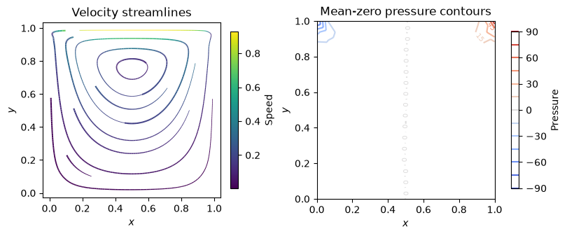
流线图显示速度场的方向和方腔内的回流结构, 线条颜色表示速度大小. 压力只确定到一个加法常数, 因而先减去区域平均值, 再绘制压力等势线.

The streamline plot shows the direction of the velocity field and the recirculation inside the cavity; line color indicates speed. Pressure is determined only up to an additive constant, so its domain average is removed before plotting pressure contours.

area = assemble(1*dx(domain=mesh))
mean_pressure = assemble(p_old*dx)/area
pressure_plot = Function(V_p, name='pressure')
pressure_plot.interpolate(p_old-mean_pressure)

fig, axes = plt.subplots(1, 2, figsize=(8, 3.3), constrained_layout=True)
streams = streamplot(u_old, axes=axes[0], seed=1, cmap='viridis')
_ = fig.colorbar(streams, ax=axes[0], shrink=0.82, label='Speed')
axes[0].set_title('Velocity streamlines')

contours = tricontour(pressure_plot, levels=12, axes=axes[1], cmap='coolwarm')
axes[1].clabel(contours, inline=True, fontsize=7)
_ = fig.colorbar(contours, ax=axes[1], shrink=0.82, label='Pressure')
axes[1].set_title('Mean-zero pressure contours')

for ax in axes:
    ax.set_aspect('equal')
    ax.set_xlabel('$x$')
    ax.set_ylabel('$y$')

5.5. 稳态方腔流与 Re = 1000 基准对比 Steady cavity flow and the Re = 1000 benchmark

为了观察惯性效应和底角涡结构, 下面直接求解稳态方程, 即从前面的方程中去掉时间导数, 边界条件不变, 并在 64 × 64 网格上取 Re = 1000. 离散空间仍为 Taylor–Hood 元.

Re = 1000 时非线性较强, 从零初值直接进行 Newton 迭代不收敛; 实测中 SNES 达到最大迭代次数后停止. 一个简单有效的补救是 Reynolds 数延拓: 依次求解 Re = 100, 400, 1000, 并以前一个 Reynolds 数的解作为下一个的初值, 使每次 Newton 迭代都从较好的初值出发. 线性求解采用前面直接法小节的 MUMPS 参数; 迭代法小节的 PCD 配置在 Re ≥ 400 时外层 FGMRES 超过 100 次仍不收敛, 这里不再使用. 对高 Reynolds 数有效的迭代法见下面的进阶内容.

To expose the inertial effects and the bottom-corner vortex structures, we now solve the steady equations directly: the time derivative is dropped from the equations above, the boundary conditions are unchanged, and we take Re = 1000 on a 64 × 64 mesh. The Taylor–Hood pair is retained.

At Re = 1000 the nonlinearity is strong, and Newton iteration started from a zero initial guess does not converge; in our tests SNES stops after reaching its iteration limit. A simple and effective remedy is Reynolds-number continuation: solve for Re = 100, 400, 1000 in turn, using the solution at the previous Reynolds number as the initial guess for the next, so that every Newton iteration starts from a good initial guess. The linear solves use the MUMPS parameters from the direct-method subsection above; the PCD configuration of the iterative-method subsection fails to converge within 100 outer FGMRES iterations for Re ≥ 400 and is not used here. See the advanced block below for an iterative method that remains effective at high Reynolds numbers.

进阶: 高 Reynolds 数的迭代法 Advanced: iterative methods at high Reynolds numbers

实验表明, 即使把 PCD 配置中的速度块换成精确的 LU 分解, Re = 1000 的稳态问题仍无法在数百次外层迭代内收敛: 瓶颈是 PCD 对 Schur 补的交换子近似随 Reynolds 数升高而退化, 放宽容差和迭代预算只能把适用范围推到约 Re = 400.

对高 Reynolds 数更稳健的是增广 Lagrangian (augmented Lagrangian) 预条件子 [BO06]. 在残量中加入一致的增广项 \(\gamma(\nabla\cdot\boldsymbol u,\nabla\cdot\boldsymbol v)\); 真解满足 \(\nabla\cdot\boldsymbol u=0\), 因而解不变. 增广后的 Schur 补有简单近似

\[S^{-1}\approx-(1/\mathrm{Re}+\gamma)\,M_p^{-1},\]

其中 \(M_p\) 是压力质量矩阵. \(\gamma\) 越大该近似越好, 外层迭代次数几乎与 Reynolds 数无关; 代价是速度块随 \(\gamma\) 增大而病态, 需要更强的求解器. 本节规模的问题可直接用 MUMPS 分解速度块, 大规模问题则需要专门设计的多重网格 [FMW19].

按下面的方式修改残量和求解器配置, 并通过 appctx 传入缩放系数 mu \(=1/\mathrm{Re}+\gamma\); MassInvPC 用它缩放压力质量矩阵, 延拓中应随 Re 同步更新. 实测中, 64 × 64 网格上延拓 Re = 100 → 400 → 1000, 每个 Newton 步只需 2–4 次外层 FGMRES 迭代, 且结果对 \(\gamma\in[10^2,10^4]\) 不敏感.

Experiments show that even replacing the velocity block of the PCD configuration by an exact LU factorization does not make the steady problem at Re = 1000 converge within hundreds of outer iterations: the bottleneck is that the commutator approximation of the Schur complement underlying PCD deteriorates as the Reynolds number grows, and relaxing tolerances and iteration budgets only extends the usable range to about Re = 400.

A more robust choice at high Reynolds numbers is the augmented Lagrangian preconditioner [BO06]. Add the consistent augmentation term \(\gamma(\nabla\cdot\boldsymbol u,\nabla\cdot\boldsymbol v)\) to the residual; the exact solution satisfies \(\nabla\cdot\boldsymbol u=0\), so the solution is unchanged. The Schur complement of the augmented system has the simple approximation

\[S^{-1}\approx-(1/\mathrm{Re}+\gamma)\,M_p^{-1},\]

where \(M_p\) is the pressure mass matrix. The larger \(\gamma\), the better this approximation, and the number of outer iterations becomes almost independent of the Reynolds number; the price is that the velocity block grows increasingly ill conditioned with \(\gamma\) and requires a stronger solver. At the scale of this section the velocity block can be factorized directly by MUMPS, whereas large-scale problems require specially designed multigrid methods [FMW19].

Modify the residual and the solver configuration as follows, and pass the scaling coefficient mu \(=1/\mathrm{Re}+\gamma\) through appctx; MassInvPC uses it to scale the pressure mass matrix, and it should be updated together with Re during continuation. In our tests on the 64 × 64 mesh with continuation Re = 100 → 400 → 1000, each Newton step needs only 2–4 outer FGMRES iterations, and the results are insensitive to \(\gamma\in[10^2,10^4]\).

gamma = Constant(1e3)
residual_al = residual + gamma*div(u)*div(v)*dx  # 增广项
mu = Constant(1.0)  # 取值 1/Re + gamma, 延拓中随 Re 更新

al_parameters = {
    'snes_error_if_not_converged': True,
    'mat_type': 'nest',
    'ksp_type': 'fgmres',
    'ksp_rtol': 1e-8,
    'pc_type': 'fieldsplit',
    'pc_fieldsplit_type': 'schur',
    'pc_fieldsplit_schur_fact_type': 'full',
    'fieldsplit_0_ksp_type': 'preonly',
    'fieldsplit_0_pc_type': 'lu',
    'fieldsplit_0_pc_factor_mat_solver_type': 'mumps',
    'fieldsplit_1_ksp_type': 'preonly',
    'fieldsplit_1_pc_type': 'python',
    'fieldsplit_1_pc_python_type': 'firedrake.MassInvPC',
    'fieldsplit_1_Mp_ksp_type': 'preonly',
    'fieldsplit_1_Mp_pc_type': 'lu',
}

solver_al = NonlinearVariationalSolver(
    NonlinearVariationalProblem(residual_al, state, bcs=bcs),
    nullspace=nullspace, solver_parameters=al_parameters,
    appctx={'mu': mu},
)
# 每次 Re.assign(...) 后同步更新: mu.assign(1/re_value + float(gamma))

solve_steady_cavity 将网格、空间、变分问题和求解器的构造封装在一起, 并依次完成延拓序列. 实测中, 三个 Reynolds 数的 Newton 迭代次数分别为 4, 5, 6.

solve_steady_cavity encapsulates construction of the mesh, spaces, variational problem, and solver, and then performs the continuation sequence. In our tests, the Newton iteration counts for the three Reynolds numbers are 4, 5, and 6.

def solve_steady_cavity(N, reynolds_numbers, solver_parameters,
                        degree=2, options_prefix='steady_ns'):
    mesh = UnitSquareMesh(N, N)
    velocity_space = VectorFunctionSpace(mesh, 'CG', degree)
    pressure_space = FunctionSpace(mesh, 'CG', degree-1)
    mixed_space = velocity_space * pressure_space

    state = Function(mixed_space, name='steady cavity state')
    u, p = split(state)
    v, q = TestFunctions(mixed_space)
    Re = Constant(1.0)
    residual = (
        1/Re*inner(grad(u), grad(v))*dx
        + 0.5*inner(dot(grad(u), u), v)*dx
        - 0.5*inner(dot(grad(v), u), u)*dx
        - p*div(v)*dx + q*div(u)*dx
    )

    bcs = [
        DirichletBC(mixed_space.sub(0), Constant((0.0, 0.0)),
                    (1, 2, 3)),
        DirichletBC(mixed_space.sub(0), Constant((1.0, 0.0)), 4),
    ]
    nullspace = MixedVectorSpaceBasis(
        mixed_space, [mixed_space.sub(0),
                      VectorSpaceBasis(constant=True, comm=mesh.comm)]
    )
    problem = NonlinearVariationalProblem(residual, state, bcs=bcs)
    parameters = dict(solver_parameters)
    parameters.setdefault('snes_max_it', 30)
    solver = NonlinearVariationalSolver(
        problem, options_prefix=options_prefix, nullspace=nullspace,
        solver_parameters=parameters,
        appctx={'state': state, 'Re': Re, 'velocity_space': 0},
    )
    newton_counts = []
    for reynolds in reynolds_numbers:
        Re.assign(reynolds)
        solver.solve()
        newton_counts.append(solver.snes.getIterationNumber())
        PETSc.Sys.Print(
            f'Re = {reynolds:6g}: Newton iterations = {newton_counts[-1]}'
        )
    return mesh, state, newton_counts


mesh_cavity, state_cavity, newton_counts = solve_steady_cavity(
    N=64, reynolds_numbers=(100, 400, 1000),
    solver_parameters=direct_parameters, options_prefix='cavity_ns',
)
velocity_cavity, pressure_cavity = state_cavity.subfunctions
assert all(count <= 10 for count in newton_counts)

Re =    100: Newton iterations = 4
Re =    400: Newton iterations = 5
Re =   1000: Newton iterations = 6

5.5.1. 流函数后处理 Streamfunction post-processing

二维不可压速度场可用流函数 \(\psi\) 描述:

A two-dimensional incompressible velocity field can be described by a streamfunction \(\psi\):

(5.7)\[\begin{equation} \boldsymbol u=\left(\frac{\partial\psi}{\partial y}, -\frac{\partial\psi}{\partial x}\right),\qquad -\Delta\psi=\omega:=\frac{\partial u_2}{\partial x} -\frac{\partial u_1}{\partial y}. \end{equation}\]

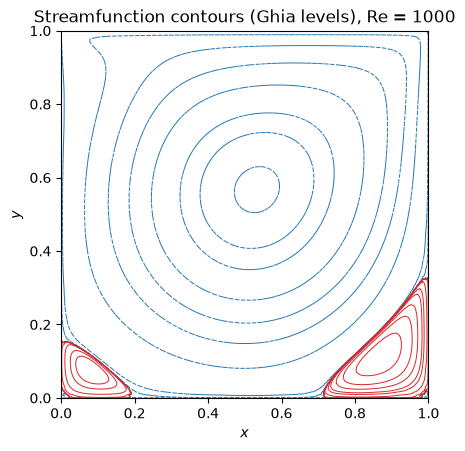
其中 \(\omega\) 是涡量. 方腔四条边都是流线, 可在整个边界上取 \(\psi=0\), 因而 \(\psi\) 由以涡量为源项的 Poisson 问题确定. 下面在二次 Lagrange 空间中求解该问题, 并按 Ghia 等人 [GGS82] 图中的层级绘制 \(\psi\) 等值线: 负层级显示顺时针旋转的主涡, 幅值很小的正层级显示两个底角的次级涡.

Here \(\omega\) is the vorticity. All four cavity walls are streamlines, so \(\psi=0\) may be imposed on the whole boundary, and \(\psi\) is then determined by a Poisson problem with the vorticity as source. We solve this problem in the quadratic Lagrange space and draw the contours of \(\psi\) at the levels used in the figures of Ghia et al. [GGS82]: the negative levels display the clockwise primary vortex, while the small positive levels reveal the secondary vortices in the two bottom corners.

def compute_streamfunction(velocity):
    mesh = velocity.function_space().mesh()
    V_psi = FunctionSpace(mesh, 'CG', 2)
    psi = Function(V_psi, name='streamfunction')
    phi = TestFunction(V_psi)
    psi_trial = TrialFunction(V_psi)
    vorticity = velocity[1].dx(0) - velocity[0].dx(1)
    a_psi = inner(grad(psi_trial), grad(phi))*dx
    L_psi = vorticity*phi*dx
    bc_psi = DirichletBC(V_psi, 0, 'on_boundary')
    solve(a_psi == L_psi, psi, bcs=bc_psi, solver_parameters={
        'ksp_type': 'preonly', 'pc_type': 'lu',
        'pc_factor_mat_solver_type': 'mumps',
    })
    return psi


psi_cavity = compute_streamfunction(velocity_cavity)

# Streamfunction contour levels used by Ghia et al. (1982)
ghia_levels_negative = [
    -0.1175, -0.115, -0.11, -0.1, -0.09, -0.07, -0.05,
    -0.03, -0.01, -1e-4, -1e-5, -1e-7, -1e-10,
]
ghia_levels_positive = [
    1e-8, 1e-7, 1e-6, 1e-5, 5e-5, 1e-4,
    2.5e-4, 5e-4, 1e-3, 1.5e-3, 3e-3,
]

fig, ax = plt.subplots(figsize=(4.6, 4.4), constrained_layout=True)
tricontour(psi_cavity, axes=ax, levels=ghia_levels_negative,
           colors='tab:blue', linewidths=0.7)
tricontour(psi_cavity, axes=ax, levels=ghia_levels_positive,
           colors='tab:red', linewidths=0.7)
ax.set_aspect('equal')
ax.set_xlabel('$x$')
ax.set_ylabel('$y$')
_ = ax.set_title('Streamfunction contours (Ghia levels), Re = 1000')

5.5.2. 涡心位置 Vortex centers

主涡中心是 \(\psi\) 的最小值点, 两个底角次级涡的中心是相应角区内 \(\psi\) 的最大值点. 下面先在给定子区域的均匀样点上粗扫, 再在最优点附近加密一次, 得到涡心位置和相应的 \(\psi\) 值, 并与 Ghia 等人 [GGS82] 的结果对比.

The primary-vortex center is the minimizer of \(\psi\), and the centers of the two bottom-corner vortices are the maximizers of \(\psi\) inside the corresponding corner regions. The code below first scans uniform sample points in a given subregion and then refines once around the best point, producing the vortex centers and the corresponding values of \(\psi\) for comparison with Ghia et al. [GGS82].

def locate_extremum(psi, kind, box, samples=61, halfwidth=0.02):
    mesh = psi.function_space().mesh()
    pick = np.argmin if kind == 'min' else np.argmax
    x0, x1, y0, y1 = box
    for _ in range(2):
        xs = np.linspace(x0, x1, samples)
        ys = np.linspace(y0, y1, samples)
        points = [(x, y) for x in xs for y in ys]
        values = PointEvaluator(mesh, points).evaluate(psi)
        best = points[pick(values)]
        x0, x1 = max(best[0]-halfwidth, 0.0), min(best[0]+halfwidth, 1.0)
        y0, y1 = max(best[1]-halfwidth, 0.0), min(best[1]+halfwidth, 1.0)
    return best, values[pick(values)]


# Ghia et al. (1982), Re = 1000: (x, y, psi) at the vortex centers
ghia_vortices = {
    'primary': (0.5313, 0.5625, -0.117929),
    'bottom right': (0.8594, 0.1094, 1.75102e-3),
    'bottom left': (0.0859, 0.0781, 2.31129e-4),
}
search_boxes = {
    'primary': ('min', (0.3, 0.8, 0.3, 0.8)),
    'bottom right': ('max', (0.6, 0.999, 0.001, 0.4)),
    'bottom left': ('max', (0.001, 0.4, 0.001, 0.4)),
}

print('vortex         x_h      y_h      psi_h       '
      'x_Ghia   y_Ghia   psi_Ghia')
for name, (kind, box) in search_boxes.items():
    (cx, cy), value = locate_extremum(psi_cavity, kind, box)
    gx, gy, gpsi = ghia_vortices[name]
    print(f'{name:13s} {cx:.4f}   {cy:.4f}   {value:10.3e}  '
          f'{gx:.4f}   {gy:.4f}   {gpsi:10.3e}')
    assert abs(cx-gx) < 0.02 and abs(cy-gy) < 0.02

vortex         x_h      y_h      psi_h       x_Ghia   y_Ghia   psi_Ghia
primary       0.5333   0.5673   -1.119e-01  0.5313   0.5625   -1.179e-01
bottom right  0.8680   0.1127    1.495e-03  0.8594   0.1094    1.751e-03
bottom left   0.0815   0.0755    1.755e-04  0.0859   0.0781    2.311e-04

5.5.3. 中线速度剖面 Centerline velocity profiles

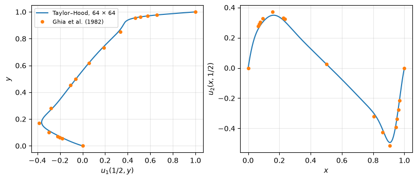
最后在 Ghia 等人 [GGS82] 表格的采样点上比较两条中线上的速度: 竖直中线 \(x=1/2\) 上的水平速度 \(u_1(1/2,y)\) 和水平中线 \(y=1/2\) 上的竖直速度 \(u_2(x,1/2)\). 下面输出对齐的对比表并绘图; 曲线为本文数值解, 圆点为 Ghia 等人的数据.

结果显示两条剖面与 Ghia 数据的最大偏差约为 0.024, 主要来自 Re = 1000 的边界层在 64 × 64 网格上的欠分辨, 以及参考数据本身的离散误差. 将 solve_steady_cavity 的 degree 提高到 3 (P3/P2 对) 或将网格加密到 128 × 128, 最大偏差可降到约 0.011.

Finally, we compare the velocities on the two centerlines at the sample points of the tables in Ghia et al. [GGS82]: the horizontal velocity \(u_1(1/2,y)\) on the vertical centerline \(x=1/2\) and the vertical velocity \(u_2(x,1/2)\) on the horizontal centerline \(y=1/2\). The code prints an aligned comparison table and plots the profiles; the curves are the present numerical solution, and the dots are the data of Ghia et al.

The results show that the maximum deviation of the two profiles from the Ghia data is about 0.024. It stems mainly from the under-resolved boundary layers at Re = 1000 on the 64 × 64 mesh, as well as from the discretization error of the reference data itself. Raising degree in solve_steady_cavity to 3 (the P3/P2 pair) or refining the mesh to 128 × 128 reduces the maximum deviation to about 0.011.

# Ghia et al. (1982), Re = 1000: u_1 on the vertical centerline x = 1/2
ghia_y = np.array([
    0.0000, 0.0547, 0.0625, 0.0703, 0.1016, 0.1719, 0.2813, 0.4531,
    0.5000, 0.6172, 0.7344, 0.8516, 0.9531, 0.9609, 0.9688, 0.9766,
    1.0000])
ghia_u = np.array([
    0.00000, -0.18109, -0.20196, -0.22220, -0.29730, -0.38289,
    -0.27805, -0.10648, -0.06080, 0.05702, 0.18719, 0.33304,
    0.46604, 0.51117, 0.57492, 0.65928, 1.00000])
# and u_2 on the horizontal centerline y = 1/2
ghia_x = np.array([
    0.0000, 0.0625, 0.0703, 0.0781, 0.0938, 0.1563, 0.2266, 0.2344,
    0.5000, 0.8047, 0.8594, 0.9063, 0.9453, 0.9531, 0.9609, 0.9688,
    1.0000])
ghia_v = np.array([
    0.00000, 0.27485, 0.29012, 0.30353, 0.32627, 0.37095, 0.33075,
    0.32235, 0.02526, -0.31966, -0.42665, -0.51550, -0.39188,
    -0.33714, -0.27669, -0.21388, 0.00000])

u_profile = PointEvaluator(
    mesh_cavity, [(0.5, y) for y in ghia_y]
).evaluate(velocity_cavity)[:, 0]
v_profile = PointEvaluator(
    mesh_cavity, [(x, 0.5) for x in ghia_x]
).evaluate(velocity_cavity)[:, 1]

print('vertical centerline x = 1/2       '
      'horizontal centerline y = 1/2')
print('      y       u_h   u_Ghia     diff  '
      '      x       v_h   v_Ghia     diff')
for i in range(len(ghia_y)):
    print(f' {ghia_y[i]:6.4f}  {u_profile[i]:8.5f} {ghia_u[i]:8.5f} '
          f'{u_profile[i]-ghia_u[i]:8.5f}   {ghia_x[i]:6.4f}  '
          f'{v_profile[i]:8.5f} {ghia_v[i]:8.5f} '
          f'{v_profile[i]-ghia_v[i]:8.5f}')
max_du = np.max(np.abs(u_profile-ghia_u))
max_dv = np.max(np.abs(v_profile-ghia_v))
print(f'max |u_h-u_Ghia| = {max_du:.4f}, '
      f'max |v_h-v_Ghia| = {max_dv:.4f}')
assert max_du < 0.03 and max_dv < 0.03

line = np.linspace(0.0, 1.0, 201)
u_curve = PointEvaluator(
    mesh_cavity, [(0.5, y) for y in line]
).evaluate(velocity_cavity)[:, 0]
v_curve = PointEvaluator(
    mesh_cavity, [(x, 0.5) for x in line]
).evaluate(velocity_cavity)[:, 1]

fig, axes = plt.subplots(1, 2, figsize=(8, 3.4), constrained_layout=True)
axes[0].plot(u_curve, line, label='Taylor–Hood, 64 × 64')
axes[0].plot(ghia_u, ghia_y, 'o', markersize=4,
             label='Ghia et al. (1982)')
axes[0].set_xlabel('$u_1(1/2, y)$')
axes[0].set_ylabel('$y$')
axes[1].plot(line, v_curve)
axes[1].plot(ghia_x, ghia_v, 'o', markersize=4)
axes[1].set_xlabel('$x$')
axes[1].set_ylabel('$u_2(x, 1/2)$')
axes[0].legend(fontsize=8)
for ax in axes:
    ax.grid(alpha=0.3)

vertical centerline x = 1/2       horizontal centerline y = 1/2
      y       u_h   u_Ghia     diff        x       v_h   v_Ghia     diff
 0.0000  -0.00000  0.00000 -0.00000   0.0000   0.00000  0.00000  0.00000
 0.0547  -0.16490 -0.18109  0.01619   0.0625   0.25426  0.27485 -0.02059
 0.0625  -0.18410 -0.20196  0.01786   0.0703   0.26890  0.29012 -0.02122
 0.0703  -0.20285 -0.22220  0.01935   0.0781   0.28175  0.30353 -0.02178
 0.1016  -0.27382 -0.29730  0.02348   0.0938   0.30360  0.32627 -0.02267
 0.1719  -0.36154 -0.38289  0.02135   0.1563   0.34839  0.37095 -0.02256
 0.2813  -0.26616 -0.27805  0.01189   0.2266   0.31516  0.33075 -0.01559
 0.4531  -0.10154 -0.10648  0.00494   0.2344   0.30756  0.32235 -0.01479
 0.5000  -0.05793 -0.06080  0.00287   0.5000   0.02626  0.02526  0.00100
 0.6172   0.05479  0.05702 -0.00223   0.8047  -0.30065 -0.31966  0.01901
 0.7344   0.17970  0.18719 -0.00749   0.8594  -0.40481 -0.42665  0.02184
 0.8516   0.31735  0.33304 -0.01569   0.9063  -0.49343 -0.51550  0.02207
 0.9531   0.45107  0.46604 -0.01497   0.9453  -0.37752 -0.39188  0.01436
 0.9609   0.49839  0.51117 -0.01278   0.9531  -0.32612 -0.33714  0.01102
 0.9688   0.56538  0.57492 -0.00954   0.9609  -0.26940 -0.27669  0.00729
 0.9766   0.65223  0.65928 -0.00705   0.9688  -0.20905 -0.21388  0.00483
 1.0000   1.00000  1.00000  0.00000   1.0000   0.00000  0.00000  0.00000
max |u_h-u_Ghia| = 0.0235, max |v_h-v_Ghia| = 0.0227

References

[BO06] (1,2)

Michele Benzi and Maxim A. Olshanskii. An augmented Lagrangian-based approach to the Oseen problem. SIAM Journal on Scientific Computing, 28(6):2095–2113, 2006. doi:10.1137/050646421.

[FMW19] (1,2)

Patrick E. Farrell, Lawrence Mitchell, and Florian Wechsung. An augmented Lagrangian preconditioner for the 3D stationary incompressible Navier–Stokes equations at high Reynolds number. SIAM Journal on Scientific Computing, 41(5):A3073–A3096, 2019. doi:10.1137/18M1219370.

[GGS82] (1,2,3,4,5,6)

U. Ghia, K. N. Ghia, and C. T. Shin. High-Re solutions for incompressible flow using the Navier–Stokes equations and a multigrid method. Journal of Computational Physics, 48(3):387–411, 1982. doi:10.1016/0021-9991(82)90058-4.